Join Optimization in Snowflake: The Power of Bloom Filters

No matter whether we are working with ***Snowflake, [Databricks](https://www.databricks.com/) or any other platform, we love visibility into query execution! And there comes [Query Profile](https://docs.snowflake.com/en/user-guide/ui-snowsight-activity)*** which can help us visualizing the details of a query execution. The query profile helps you troubleshoot performance bottlenecks during the query’s execution. For example:

• You can visualize each query operator and related metrics, such as the time spent, number of rows processed, rows processed, and memory consumption.
• You can identify the slowest part of a query execution at a glance and assess the impacts of modifications to the query.
• You can discover and fix common mistakes in SQL statements, such as exploding joins or full table scans.

One day I was just casually exploring query profile for the last query in the below code & found 2not so obvious steps in it —

ALTER SESSION SET USE_CACHED_RESULT = FALSE;

create or replace database demo_test;

use demo_test;

-- Departments (T2) — 1 row per department
CREATE TABLE departments (
  dept_id   INT,
  dept_name VARCHAR(20)
);
INSERT INTO departments VALUES
(1, 'Engineering'),
(2, 'Marketing');

-- Employees (T1) — many rows per department
CREATE TABLE employees (
  emp_id   INT,
  dept_id  INT,
  salary   DECIMAL(10,2)
);
INSERT INTO employees VALUES
(1, 1, 60000),
(2, 1, 75000),   -- Engineering has 4 employees
(3, 1, 90000),
(4, 1, 55000),
(5, 2, 50000),   -- Marketing has 3 employees
(6, 2, 62000),
(7, 2, 48000);

SELECT d.dept_name, SUM(e.salary)
FROM   employees e
JOIN   departments d ON e.dept_id = d.dept_id
GROUP  BY d.dept_name;

The Intuitive Query Profile:

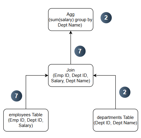
The actual Query Profile & strange steps:

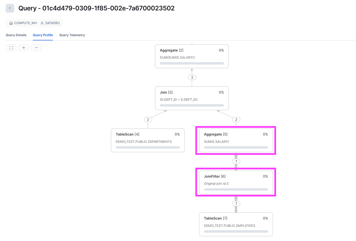
There are 2 highlighted steps performed in the Employees table(note: this is the bigger table in this case) side before performing actual join with Departments table(note: smaller table in this case) — A JoinFilter step & an Aggregate step 🤔

In case you are curious to know why actual aggregation is happening before join, then I have already covered this in ***this blog, in short, it’s an optimization which is known as Aggregate Pushdown***!

Now let’s try to understand the mystery behind the JoinFilter Step.

Prerequisite:

Before jumping further, it’s recommended to have an in-depth intuiton of Bloom Filter concept —

[embed]

In short, Bloom filters are a space-efficient probabilistic data structure that supports adding elements and checking whether specific elements were previously added. It trades absolute precision for massive memory savings by answering one of two things: an item is “definitely not in the set” or “possibly in the set”

Also, you can understand & visualize the next steps much better if you have clear understanding on internals of Join in Distributed system which is covered ***here***.

Now let’s discuss, how Bloom Filter can be used to improve the Join Operation also in some cases, let’s see how..

Bloom Filter Join:

Let’s say we have to inner join a Dimension table & Fact Table(remember, in general, Dimension Table size is generally much smaller than Fact Table)—

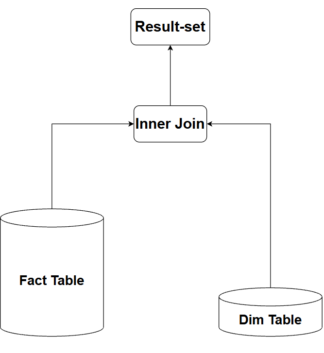
Now, regardless of whether we use a Broadcast Join, Shuffle Hash Join, or Sort Merge Join, the large fact table will still result in significant computation. So the real question is: Can we reduce the number of rows entering the join operation in the first place?

Solution: We know we are going to do Inner Join, that means we don’t need the keys from Fact Table which are not available in Dim Table! So what if we do like this —

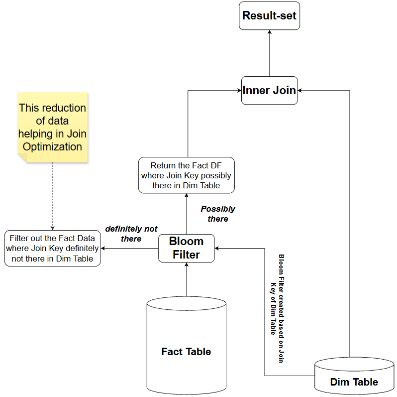
Bloom join

So the idea is simple: build a Bloom Filter from the Dimension Table’s join keys and apply it to the Fact Table before the join. Any row that fails the filter is guaranteed not to have a matching key in the Dimension Table and can be discarded immediately. Only rows that might have a match proceed to the join, significantly reducing the amount of data that needs to be processed.

Why does this help? Because checking a row against a Bloom Filter is far cheaper than sending that row through an expensive join operation. By quickly filtering out rows that definitely have no match, the query engine reduces the amount of data participating in the join, leading to faster execution and lower compute costs.

Modern OLAP DBMSs like Snowflake use this technique to optimize complex join operation & that step is known as JoinFilter!

Some intuition around Query Profile shown earlier:

As discussed earlier, a Bloom Filter is usually created from the smaller table’s join keys and then applied to the larger table. In our example, we can see that the JoinFilter is being applied to the larger Employee table, indicating that it was likely built from the smaller Department table. This behavior matches exactly what we would expect based on the Bloom Filter join optimization technique.

Bloom Filter in Outer Join Case:

Let’s intuitively understand whether a Bloom Filter can be applied to the following query pattern:

fact_table left join dim table on fact_table.key = dim_table.key

Unlike an Inner Join, a Left Outer Join must return all rows from the Fact Table, regardless of whether a matching key exists in the Dimension Table. Any non-matching rows simply receive NULL values for the Dimension Table columns.

Because every Fact Table row must be preserved, we cannot use a Bloom Filter built from the Dimension Table to eliminate rows from the Fact Table before the join. Doing so would change the query result and violate the semantics of the Left Outer Join.

As a result, the classic Bloom Filter-based Join Filter optimization that we discussed for Inner Joins is generally not applicable in this scenario. Since there is no opportunity to safely discard Fact Table rows, creating and applying a Bloom Filter would provide little to no benefit!

Experimentation:

SELECT
    e.emp_id,
    d.dept_name
FROM employees e
LEFT JOIN departments d
    ON e.dept_id = d.dept_id;

Query Profile:

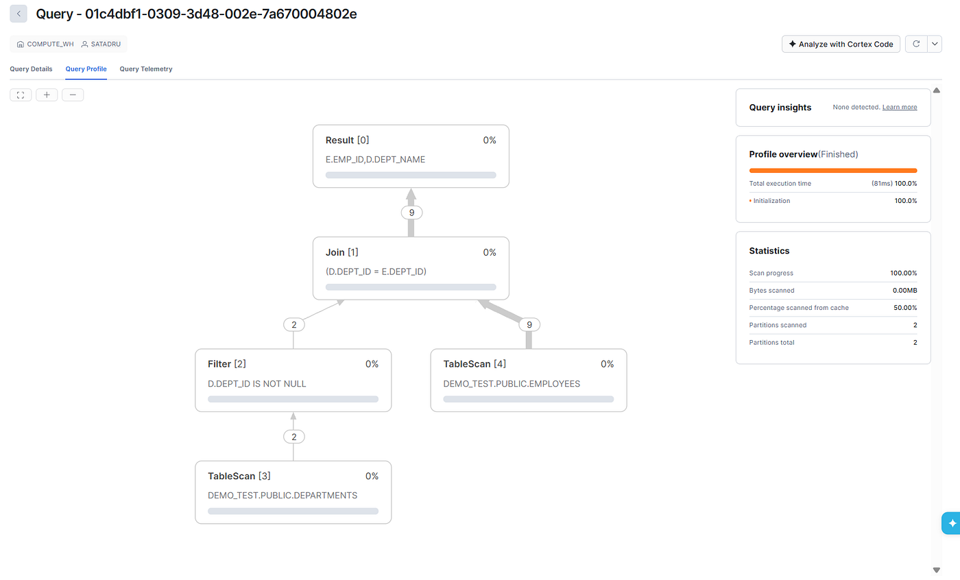
As we can see in above Query Profile, there is no JoinFilter!

Conclusion

In this blog, we demystified one of the less obvious yet powerful optimization techniques used by modern query engine, Snowflake— the Join Filter. We saw how a simple probabilistic data structure can significantly reduce the amount of data participating in a join, leading to faster and more efficient query execution.

For more such interesting and practical contents, follow me on ***YouTube, [LinkedIn](https://www.linkedin.com/in/satadru-mukherjee-a237b41a5/)*, and Medium**!