The Compilation Wall: Why Non-NVIDIA Chips Pay a Hidden Tax on Every Inference Optimization

A low-level look at why Midjourney left TPUs, Liquid AI abandoned JAX, and what it means for the future of AI accelerators.

Two Escape Stories

In March 2023, Google Cloud proudly announced that Midjourney — one of the most recognizable AI image generation platforms in the world — had chosen TPUs to train its fourth-generation model. David Holz, Midjourney’s founder, confirmed they were “training the fourth version of our algorithm on the latest v4 TPUs with JAX.” It seemed like a validation of Google’s hardware-framework thesis: build the chip, build the framework, and users will come.

Two years later, Holz told the world on X that the decision “set Midjourney’s research progress back by a full year.”

A year isn’t a rounding error in the AI race. It’s the difference between leading a generation and chasing one. Midjourney didn’t leave because TPUs were slow in benchmarks. They left because the entire development experience — the iteration speed, the tooling friction, the ecosystem gaps — made their team slower than competitors running on NVIDIA hardware with PyTorch.

Around the same time, a different story was playing out at Liquid AI. In mid-2023, the startup began training foundation models on AWS A100 GPU clusters using JAX. The choice seemed obvious: JAX offered built-in scan operations critical to their state-space model architecture, superior JIT compilation, and accessible model sharding via pjit.

Three months in, they hit a wall — literally. Multi-node training on two nodes was slower than a single node. They needed four nodes just to break even. The root cause? The NCCL version bundled with their JAX installation wasn’t compatible with AWS’s EFA interconnect. Cross-node bandwidth had dropped by 100×.

The kicker: when they implemented the same bandwidth test in PyTorch, it worked perfectly. Full cross-node bandwidth, zero configuration needed. Same GPUs, same cluster, same interconnect. Different framework, different result.

They ported their entire training stack to PyTorch in two days. “PyTorch eager mode matched JAX JIT performance on our workloads on single-node runs,” wrote co-founder Mathias Lechner — a finding that was, as he noted, “disappointing for JAX.”

These are not isolated incidents. They are two manifestations of the same structural problem, hitting at different layers of the stack:

• Midjourney hit the wall at the programming model and ecosystem layers — the accumulated friction of developing on TPU+JAX made them slower than the competition.
• Liquid AI hit the wall at the communication layer — a framework-specific incompatibility made multi-node training nonfunctional.

Both companies escaped. Both lost months. And both arrived at the same destination: NVIDIA GPUs + PyTorch.

I call the structure they collided with the Compilation Wall.

What Is the Compilation Wall?

The AI accelerator landscape today offers four distinct execution models. Understanding their differences is essential to understanding why some teams thrive and others stumble.

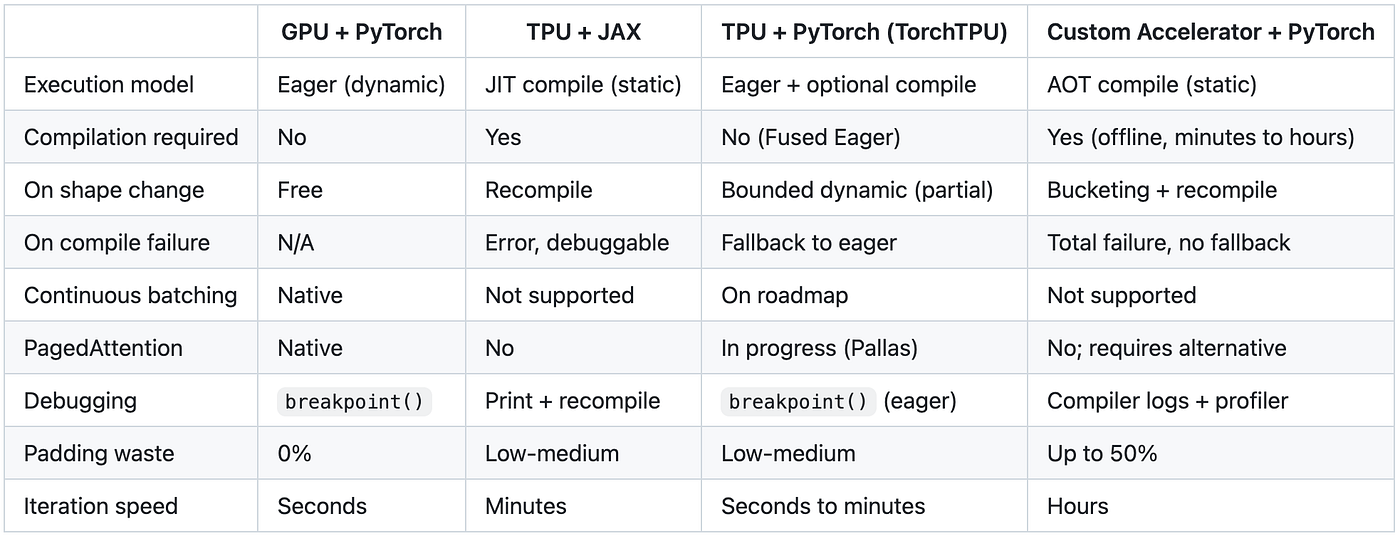
The Compilation Wall is not a single barrier. It manifests across three distinct layers:

Layer 1: Communication infrastructure. Multi-device collective operations fail or degrade when the framework’s communication library isn’t tightly integrated with the hardware interconnect. This is what killed Liquid AI’s JAX+NCCL+EFA stack.

Layer 2: Programming model constraints. The static graph compiler rejects operations it cannot handle — dynamic shapes, Python control flow, irregular memory access patterns. Engineers must restructure their code around compiler limitations rather than writing natural PyTorch.

Layer 3: Ecosystem and community. When something breaks, there’s no Stack Overflow answer, no GitHub issue with a workaround, no community-maintained library that already solved it.

The wall’s height varies by platform:

• GPU + PyTorch: No wall. Write it, run it, debug it.
• TPU + TorchTPU: A short wall. Eager mode works; compilation is optional for performance.
• TPU + JAX: A medium wall. Compilation is mandatory, but Google’s internal community provides support.
• Custom accelerators: A tall wall. Offline compilation is mandatory, there’s no fallback on failure, and the community is minimal.

As PyTorch/XLA’s own documentation states: “Graph compilations in XLA are pretty expensive. XLA handles static shape only — even for the same IR graph, XLA recompiles when input shape changes.” Even more telling: “XLA now has pretty good bounded dynamic shapes coverage already, but we still see recompilations and they are expected.”

The compilation wall doesn’t just slow you down once. It taxes every optimization you try to build.

• The Compilation Wall (n.): The aggregate cost — across communication, compilation, and ecosystem layers — of every engineering decision that must be made differently, or every optimization that cannot be applied at all, because the software/hardware stack requires static graph compilation rather than dynamic execution.

Deep Dive: The Execution Model Spectrum

To understand why the compilation wall exists at different heights for different platforms, we need to look at how each system actually executes operations at the hardware level.

GPU: True Eager — Instruction-Stream Processing

When you write a = torch.matmul(x, w) on a GPU, here's what happens at the hardware level:

1. Python calls into PyTorch’s C++ dispatcher (~1μs)
2. Dispatcher identifies the CUDA kernel for matmul
3. Kernel is submitted to the GPU’s Command Processor via the CUDA driver
4. Command Processor places it in the hardware instruction queue
5. Streaming Multiprocessors (SMs) execute the kernel
6. Result is available in GPU HBM

Total latency: ~5–10 microseconds per operation. The GPU’s Command Processor is designed to accept arbitrary kernels one at a time, in any order. It never needs to see “the whole plan” — it just executes whatever arrives next in the queue.

This is why eager mode works so well on GPUs: the hardware is an instruction-stream processor. Submitting one kernel at a time is its native operating mode.

TPU + TorchTPU: Pseudo-Eager — Micro-Batch Compilation

TorchTPU’s “Fused Eager” is fundamentally different from GPU eager, despite looking similar to the user:

# What the user writes (looks like eager):
a = torch.matmul(x, w)      # → TorchTPU runtime buffers this op
b = torch.relu(a)            # → buffers this op  
c = b + bias                 # → buffers this op
                             # → runtime detects fusible pattern
                             # → compiles [matmul, relu, add] into one XLA kernel (~1-5ms)
                             # → submits to TPU
                             # → result available

The key mechanism is the Operation Stream Observer: TorchTPU’s runtime watches the sequence of operations being dispatched, identifies patterns it can fuse (e.g., linear + activation, attention blocks), checks its Compilation Cache for a previously compiled version, and either reuses the cached binary or triggers a fast micro-compilation.

Why can micro-graphs compile in milliseconds when full models take minutes? Because a 3–10 op subgraph has trivial shape inference, doesn’t need cross-layer memory planning, and XLA maintains pre-optimized templates for common patterns like matmul+activation fusions.

The result: ~5–10 millisecond latency per fused group, compared to ~5–10 microseconds on GPU. That’s 1000× slower per operation — but for a training step that takes hundreds of milliseconds total, this overhead is imperceptible. And critically, print(tensor) works at any point: it triggers a flush of the current operation buffer, compiles and executes whatever has accumulated, and returns real values.

TPU + JAX: Function-Level Compilation

JAX’s @jit decorator traces an entire function into a static HLO graph on first call, compiles it via XLA (typically seconds to minutes depending on graph size), then caches the compiled binary for subsequent calls with the same input shapes.

@jax.jit
def forward(x, w, bias):
    a = jnp.matmul(x, w)    # ← not executed; just traced
    b = jax.nn.relu(a)       # ← not executed; just traced  
    return b + bias          # ← not executed; just traced
# First call: trace + compile + execute (seconds)
# Subsequent calls: execute only (fast)
# Shape change: full recompile (seconds again)

The compiler has a global view of the entire function, enabling aggressive optimizations: operator fusion, communication-computation overlap, SBUF/HBM memory planning. But the cost is rigidity — the function must be pure (no side effects), shapes must be static, and any shape change triggers expensive recompilation.

Custom Accelerators (Neuron, etc.): Full-Graph AOT Compilation

At the far end of the spectrum, some accelerators require the entire model to be compiled offline before any inference can happen:

# Offline compilation (minutes to hours):
compile(model, shapes=[(1,128), (1,256), (1,512), (1,1024)])
→ Generates one binary (NEFF) per shape
→ Each binary contains:
    - Exact SBUF allocation for every tensor at every timestep
    - Exact DMA schedule (which data moves when)
    - Exact compute schedule (which engine does what, when)
    - All three engines pipelined at clock-cycle granularity

# Runtime: select binary + pad + execute
input_300_tokens → pad to 512 → load 512-shape binary → execute

The hardware doesn’t have a command processor or instruction queue in the GPU sense. It’s a dataflow processor — you load a complete execution plan, feed data in one end, and results come out the other. Like burning a bitstream onto an FPGA: incredibly efficient once loaded, but you can’t dynamically insert a new operation mid-execution.

This is why these systems achieve the highest raw efficiency (zero dispatch overhead, perfect pipeline utilization) but impose the tallest compilation wall (no eager mode is architecturally possible).

The Fundamental Tradeoff

These four models form a spectrum that reveals an inherent engineering tradeoff:

Compiler's global knowledge:     Low ◄────────────────────► High
Hardware efficiency:              Low ◄────────────────────► High  
Developer freedom:               High ◄────────────────────► Low
Compilation wall height:          None ◄────────────────────► Tall

                          GPU     TorchTPU    JAX JIT    AOT Compile
                         Eager   Fused Eager  Function    Full Graph

The more the compiler knows about your computation (larger graph, static shapes, known memory layout), the better it can optimize. But the more it needs to know, the more constrained you are as a developer — and the taller the compilation wall becomes.

GPU eager sits at one extreme: the compiler knows nothing beyond the current operation, so it can’t optimize across ops, but you can write literally anything and it runs immediately. Full-graph AOT compilation sits at the other: the compiler knows everything, optimizes perfectly, but demands total rigidity.

TorchTPU’s Fused Eager is Google’s attempt to find a middle ground — giving the compiler enough visibility to fuse common patterns while preserving the “write and run” developer experience. Whether this middle ground is close enough to GPU eager to attract developers back to TPUs remains the open question.

How TorchTPU Fakes Eager (When the Hardware Can’t Do It)

The TPU cannot execute a single operation on demand the way a GPU can. It has no command processor that accepts arbitrary one-off kernels. So how does TorchTPU make it feel like eager? Three tricks working in concert:

Trick 1: Implicit synchronization (no manual sync() needed).

The old PyTorch/XLA forced users to manually call xm.mark_step() or torch_xla.sync() to trigger compilation and execution. Forget that call, and your print(tensor) would show a placeholder, not a real value. TorchTPU eliminates this: the runtime automatically flushes the operation buffer whenever you access a tensor's value — .item(), print(), passing to CPU, or reaching a training step boundary. From the user's perspective, values are "always there" when you need them.

Trick 2: Compilation cache turns cold starts into a one-time cost.

The first training step pays for compilation — the runtime sees new operation patterns, compiles micro-graphs via XLA, and caches them keyed by (operation sequence, input shapes). From the second step onward, every pattern hits the cache. Compilation cost drops to zero. For training workloads where every step executes the same operation sequence, this means the “fake eager” experience converges to near-GPU-eager latency after the first iteration.

Trick 3: Asynchronous execution hides the remaining latency.

When Python dispatches an operation to TorchTPU, the call returns immediately — Python doesn’t wait for the TPU to finish. The TPU compiles and executes in the background while Python continues dispatching more operations. Only when Python actually needs a tensor’s value does it synchronize and wait. In a typical training loop, by the time optimizer.step() needs gradient values, the TPU has already finished computing them tens of milliseconds ago. The synchronization wait is zero.

Why this isn’t true eager — and why it usually doesn’t matter:

On a GPU, after a = torch.matmul(x, w), the value of a genuinely exists in GPU memory within microseconds. On TorchTPU, a might not exist yet — it's still sitting in the operation buffer, waiting to be compiled and executed. The value only materializes when something forces a synchronization.

For training loops (same ops every step, values only needed at step boundaries), this distinction is invisible. For interactive debugging (print mid-forward-pass), it adds a few milliseconds of latency — noticeable if you're timing individual operations, but perfectly fine for development. For dynamic control flow (if loss > threshold), reading the loss value forces a sync, which works correctly but may trigger fresh compilation on the new code path.

The one scenario where the illusion breaks down is iterative token generation during inference: each step may produce a different sequence length, potentially triggering recompilation on every iteration. This is precisely why Google’s roadmap prioritizes “bounded dynamism” — telling the compiler “this dimension will be between 1 and 2048” so it can compile once and handle all lengths within that range without recompiling.

Think of it like video: a screen showing 30 discrete frames per second isn’t truly continuous motion, but it fools human perception. TorchTPU’s millisecond-granularity micro-compilation isn’t truly eager execution, but it fools the developer experience. The compilation wall is still there — it’s just been sliced thin enough to slip beneath the threshold of perception.

What Google Didn’t Say: Open Questions About Fused Eager

Google’s blog post describes Fused Eager in exactly one paragraph. The full technical disclosure is a single sentence: “Using automated reflection on the stream of operations, TorchTPU fuses steps on the fly into larger, computationally dense chunks before handing them to the TPU.”

From this, we can confirm: the runtime watches the operation stream, dynamically groups operations, and compiles them as fused chunks before execution. All modes share a persistent compilation cache. And the hardware does support single-op dispatch (Debug Eager and Strict Eager prove this), meaning Fused Eager is a software optimization layer on top of hardware that can run individual ops — unlike full-graph accelerators where single-op dispatch is architecturally impossible.

But several critical details remain undisclosed:

1. What does “automated reflection” actually mean? Is it pattern matching against a library of known-fusible sequences (matmul+activation, QKV projection+attention)? Heuristic grouping based on op properties (all compute-bound, no external references to intermediates)? Profile-guided optimization that learns from the first few iterations? Some combination? The answer determines how well Fused Eager handles novel architectures versus well-known transformer patterns.

2. What is the fusion granularity? How many operations constitute a “chunk”? Three ops? Ten? An entire transformer layer? The granularity directly affects the tradeoff between compilation latency (larger chunks = slower compilation) and execution efficiency (larger chunks = more optimization opportunity).

3. What is the first-execution compilation latency? The blog claims 50–100% speedup over Strict Eager and mentions the compilation cache, but never states how long the first compilation takes. Is it 1ms? 10ms? 100ms? For training (same ops every step), this is amortized away. For inference with variable inputs, this number determines whether Fused Eager is viable at all.

4. How much performance does Fused Eager leave on the table vs. full-graph torch.compile? The blog only compares Fused Eager to Strict Eager (50–100% improvement). It never compares to full-graph compilation. If torch.compile delivers another 2× on top of Fused Eager, then Fused Eager is a development convenience, not a production solution. If the gap is only 10–20%, then most users can skip torch.compile entirely.

5. How does it handle compilation failures in the fused path? If the runtime tries to fuse a group of ops but XLA can’t compile them together, does it fall back to Strict Eager (single-op dispatch)? Or does it try smaller sub-groups? The graceful degradation behavior determines whether Fused Eager truly “just works” or whether certain op combinations will silently crater performance.

These questions will likely be answered when Google releases the public GitHub repository (promised in their 2026 roadmap). Until then, the developer community is left evaluating TorchTPU based on a single blog post and the theoretical foundation of the 2021 LazyTensor paper — a gap that understandably fuels skepticism among teams burned by previous TPU integration promises.

The Hidden Tax: Four Case Studies

The compilation wall isn’t theoretical. Here’s what it looks like in production inference systems.

Case A: The O(n²) Transfer Problem

On GPUs, FlashAttention fuses the attention mask logic directly into the CUDA kernel. The mask never exists as a tensor — it’s computed on-the-fly inside the kernel, with zero transfer cost.

On a static-graph accelerator, the attention mask must be an explicit input tensor to the compiled graph. For a vision-language model processing 16K vision tokens, this means transferring a [16384, 16384] boolean tensor — roughly 512MB — from CPU to device on every forward pass.

In our profiling of a production vision encoder on a static-graph accelerator, this single transfer consumed over 600ms, accounting for 40% of the total forward pass latency.

The fix? Don’t transfer the mask. Transfer a 1D position ID vector (64KB) instead, and reconstruct the 2D mask on-device with a single broadcast comparison:

mask = (position_ids.unsqueeze(1) == position_ids.unsqueeze(0))

This reduced transfer time from 600ms to under 1ms — an optimization that GPU engineers never need to think about, because FlashAttention already solved it at the kernel level.

The tax: On static-graph hardware, engineers must manually design compact representations for every large tensor and implement on-device reconstruction. On GPUs, the kernel handles it.

Case B: The Padding Tax

Modern GPU inference engines achieve 3–5× higher throughput than naive implementations through two techniques that fundamentally require dynamic execution:

1. Continuous batching — requests enter and leave the batch at iteration boundaries, not epoch boundaries. Each iteration can process a different set of sequences.
2. PagedAttention — KV cache is allocated dynamically in non-contiguous blocks, eliminating memory fragmentation.

As the PagedAttention paper states: “To allocate physical memory dynamically, PagedAttention changes the layout of KV-cache from contiguous to non-contiguous virtual memory. One needs to rewrite the attention kernels to support paging.”

Static-graph accelerators cannot implement either technique natively:

• Continuous batching requires the batch composition to change every iteration — but each new composition is a new computational graph that requires recompilation.
• PagedAttention requires dynamic memory allocation and irregular memory access patterns — operations that static graph compilers cannot represent.

Instead, these systems use bucketing: pre-compiling the model for a fixed set of shapes (e.g., sequence lengths [128, 256, 512, 1024]). A request with 129 tokens gets padded to 256, wasting 50% of computation. In practice, bucketing wastes 20–30% of effective compute across a realistic request distribution.

The tax: 20–50% compute waste from padding, plus inability to use the industry’s most effective serving optimizations — a throughput gap of 3–5× on identical workloads.

Case C: The CPU/Device Partitioning Tax

On a GPU with PyTorch, model.forward() can contain arbitrary Python — dynamic shapes, conditional branches, variable-length loops. It all just runs.

On a static-graph accelerator, every line of code is a compiler-compatibility decision. Engineers must constantly ask: “Can the compiler handle this operation with a statically-known shape?”

• Dynamic logic (varying image count, variable resolution) → must execute on CPU
• Heavy computation (matmul, embedding lookup, attention) → must execute on device
• Wrong decision → either compilation failure or catastrophic performance

For multimodal models, this partitioning is especially painful. A vision-language model has inherently dynamic inputs — different numbers of images, different resolutions, different aspect ratios. Every piece of preprocessing logic that touches these dimensions must be carefully separated from the compiled device graph.

The tax: Every line of model code carries a hidden cognitive burden — “will the compiler accept this?” — that GPU engineers never face.

Case D: The Communication Stack Fragility

When Liquid AI ran their bandwidth test on JAX, cross-node bandwidth dropped 100×. When they ran the identical test in PyTorch, it hit full bandwidth. Same hardware.

The root cause was a three-vendor incompatibility: JAX (Google) shipped an NCCL version (NVIDIA) that didn’t work with EFA (AWS). Three companies, three competing optimization targets, zero integration testing for this specific combination.

NVIDIA’s GPU ecosystem doesn’t have this problem because NVIDIA controls both the hardware (ConnectX/InfiniBand) and the communication library (NCCL). They’re optimized together, tested together, shipped together.

Custom accelerator vendors control their own communication layer (e.g., AWS controls EFA + Neuron Runtime), so they don’t face this specific issue. But they trade it for a larger compilation-layer problem.

The tax: Outside the NVIDIA+PyTorch stack, every layer of the software stack becomes a potential point of failure — with no guarantee that the vendors involved have tested the specific combination you’re using.

Why torch.compile Doesn’t Solve This

One might argue that PyTorch itself is moving toward compilation via torch.compile. Doesn't that mean GPUs will face the same wall eventually?

No. The critical difference is fallback.

torch.compile on GPU:
  Compile succeeds → use fast compiled path
  Compile fails   → fallback to eager mode (slower, but still works)
  Dynamic shape   → graph break, partial compilation

Static-graph accelerator:
  Compile succeeds → can run
  Compile fails   → cannot run at all
  Dynamic shape   → not supported

Benchmarks confirm the trade-off: torch.compile adds 95 seconds of compilation overhead (vs. 3 seconds for eager) and performs 15% worse than TorchScript on dynamic-shape workloads. But the key insight is that on GPUs, compilation is optional. It's a performance optimization, not a correctness requirement.

On static-graph accelerators, compilation is the only path to execution. There is no fallback. This fundamental asymmetry means that every compiler limitation becomes a hard blocker rather than a performance trade-off.

Why These Chips Still Matter

This is not a hit piece on alternative accelerators. Static graph compilation has genuine advantages — but only when the conditions are right.

The Industry’s Pivot to PyTorch — And Its Limits

The pattern is now unmistakable. Google built TorchTPU to give PyTorch users a native path to TPUs. AWS’s Neuron SDK tells a similar story: the trajectory is clear — every significant investment (NxD Inference, torch.compile integration, TorchTitan compatibility, vLLM backend) is PyTorch-exclusive. JAX remains listed as supported, but receives no comparable engineering attention. The message from every non-NVIDIA chip vendor is the same: “You don’t need to learn a new framework. Just use PyTorch.”

But here’s the uncomfortable truth: adopting PyTorch doesn’t remove the compilation wall. It only changes the entrance.

Consider what “PyTorch support” actually means on each platform:

GPU + PyTorch:       Eager execution. Write anything, run immediately.
TPU + PyTorch:       Pseudo-eager (Fused Eager). Feels like eager, compiles under the hood.
Neuron + PyTorch:    torch_neuronx. PyTorch syntax, but mandatory AOT compilation.
                     Same bucketing. Same padding waste. Same compilation hours.
                     Just with PyTorch API instead of JAX API.

Dropping JAX in favor of PyTorch solves the framework familiarity problem — engineers don’t need to learn a new language. But it does nothing for the hardware constraint problem — static shapes, mandatory compilation, no PagedAttention, no continuous batching.

It’s like switching the road signs from German to English. The road itself — narrow, with hairpin turns and no guardrails — hasn’t changed. You can now read the warnings, but you’ll still go off the cliff if you drive like you’re on a highway.

This is why AWS’s strategy diverges from Google’s. Google is trying to make the road wider (TorchTPU eager modes, bounded dynamism). AWS appears to have accepted that the road will stay narrow, and is instead building a taxi service (Bedrock, SageMaker) so users never have to drive themselves.

When Static Graph Compilation Wins

Once compiled, static-graph execution eliminates kernel launch overhead, op dispatch overhead, and Python interpreter overhead entirely. The compiler can perform global optimizations — operator fusion, communication-computation overlap, memory reuse — that are difficult or impossible in eager mode.

These advantages compound in a specific scenario: high-volume serving of fixed models. When you compile once and execute millions of times, the compilation cost is amortized to near-zero, and the per-inference efficiency advantage is real.

Each camp has chosen a different strategy to address the compilation wall:

NVIDIA (GPU + PyTorch): No wall to address. They are the standard. Ongoing investment in CUDA, Triton, and the broader ecosystem reinforces their position.

Google (TPU + TorchTPU, 2026): Lower the wall. Their new TorchTPU stack implements an “Eager First” philosophy with three execution modes, including Fused Eager (50–100% faster than strict eager). But a critical clarification: TorchTPU’s “eager” is not true per-op eager execution like GPUs. Under the hood, it’s lazy evaluation with automatic micro-graph compilation — the runtime accumulates a few operations, compiles them into a small optimized kernel in milliseconds, then executes the batch. The key difference from JAX/XLA isn’t whether it compiles — it always does — but when and how much: small graphs compiled on-the-fly in milliseconds, rather than entire models compiled ahead-of-time in minutes. The user experience feels like eager because the compilation granularity is small enough to be imperceptible. But the TPU still cannot execute a single arbitrary op without some form of compilation. The compilation wall is shorter, not absent.

Google (TPU + JAX, legacy): The strategy that Midjourney fled. Still used internally for Gemini and other Google-scale models, but no longer the recommended path for external developers.

AWS (Neuron, TorchNeuron): The same playbook. AWS’s Neuron documentation reveals a parallel effort called TorchNeuron — a native PyTorch backend for Trainium that mirrors TorchTPU’s architecture almost exactly. It uses the same PrivateUse1 device interface, supports eager mode where “operations are dispatched and execute immediately,” and implements its own version of automatic fusion called “Adaptive Eager Execution.” According to the official documentation: “TorchNeuron takes advantage of [asynchronous dispatch] by analyzing sequences of queued operators and fusing them into single operators based on fusion heuristics.” It also supports torch.compile via a custom TorchDynamo backend that lowers FX graphs to Neuron IR. The migration path is identical to TorchTPU's promise: change .to('cuda') to .to('neuron'), and the rest of your code stays the same. This represents a fundamental shift from the older torch_neuronx stack, which required offline ahead-of-time compilation with no eager fallback. The compilation wall on Neuron hardware is being actively lowered — though how much of this closes the gap with GPU eager in practice remains to be validated at scale.

The convergence is striking: Google and AWS, independently, arrived at the same architectural answer — PrivateUse1 backend, adaptive operator fusion, torch.compile integration, and the “change one line to migrate” developer promise. Both are trying to make their compilation wall short enough to be imperceptible. Whether either succeeds depends on execution details neither has fully disclosed.

Conclusion

NVIDIA’s moat is not chip performance. It’s not CUDA’s syntax. It’s not even the software ecosystem, though that helps enormously.

NVIDIA’s moat is the absence of a compilation wall.

GPU + PyTorch eager = write it, run it, debug it, ship it. No compilation step. No shape restrictions. No fallback failures. No CPU/device partitioning decisions. No padding waste. No three-vendor communication stack to debug.

Every alternative introduces a wall somewhere. The wall might be short (TorchTPU and TorchNeuron’s adaptive eager fusion) or tall (legacy static-graph stacks with mandatory AOT compilation and no fallback). But its mere existence means that engineers spend time fighting the infrastructure instead of optimizing the model.

The compilation wall won’t disappear — it’s a fundamental consequence of hardware that trades generality for efficiency. But it can be made shorter. Google and AWS, independently, are trying to shrink it with micro-graph compilation that feels like eager execution (though it isn’t, truly — these chips still compile every operation, just in smaller, faster batches). The convergence of their approaches — same interface (PrivateUse1), same technique (adaptive fusion), same promise (“change one line”) — suggests this is the only viable path forward for non-NVIDIA hardware.

NVIDIA doesn’t need to do any of this because the wall was never there.

The race in AI inference hardware is often framed as a competition over FLOPS, memory bandwidth, or price-per-token. But the real competition might be simpler:

Who can make their compilation wall invisible first?

If you’ve worked with non-NVIDIA inference hardware and have your own compilation wall stories, I’d love to hear them. The more data points the industry collects, the better we can assess which walls are shrinking and which are here to stay.