A Practical Guide to EfficientNet with Python Examples
Deep learning models have become increasingly powerful over the years. Researchers often improved performance by making networks:
A Practical Guide to EfficientNet with Python Examples

Deep learning models have become increasingly powerful over the years. Researchers often improved performance by making networks:
- Deeper (more layers)
- Wider (more channels)
- Higher resolution (larger input images)
However, simply increasing one of these dimensions often leads to inefficient use of computational resources.
This challenge led researchers at Google to introduce EfficientNet, a family of convolutional neural networks that achieved state-of-the-art accuracy while using significantly fewer parameters and FLOPs.
In this article, we’ll explore:
- Why EfficientNet was created
- The concept of Compound Scaling
- EfficientNet architecture
- EfficientNet variants (B0–B7)
- Dog breed classification example
- Python implementation using TensorFlow
The Problem with Traditional Scaling
Suppose we have a CNN that classifies dogs.
Option 1: Make it Deeper
Increase layers:
20 Layers → 50 Layers → 100 LayersBenefits:
- Learns more complex features
Problems:
- More memory
- Longer training time
- Diminishing returns
Option 2: Make it Wider
Increase channels:
64 Filters → 128 Filters → 256 FiltersBenefits:
- Captures richer features
Problems:
- Parameter count explodes
Option 3: Increase Image Resolution
Increase image size:
224×224 → 380×380 → 600×600Benefits:
- More visual detail
Problems:
- Higher computational cost
Researchers discovered that scaling only one dimension is not optimal.
The solution?
Scale all dimensions together in a balanced manner.
This idea became the foundation of EfficientNet.
What Makes EfficientNet Different?
EfficientNet introduces a technique called:
Compound Scaling
Instead of arbitrarily increasing depth, width, or resolution, EfficientNet scales them simultaneously.
Mathematically:
Depth = α^φ
Width = β^φ
Resolution = γ^φ
where:
- α controls depth
- β controls width
- γ controls resolution
- φ determines model size
Subject to:
α × β² × γ² ≈ 2This ensures computational resources are allocated efficiently.
Intuition Using Dog Breed Classification
Imagine we want to distinguish between:
- Husky
- Golden Retriever
- German Shepherd
A small model may focus on:
- General shape
- Fur color
A larger EfficientNet model learns:
More Depth
Recognizes:
- Ear structure
- Facial proportions
More Width
Learns multiple feature types simultaneously:
- Fur texture
- Eye shape
- Tail characteristics
Higher Resolution
Detects fine details:
- Fur patterns
- Nose structure
- Eye color variations
Because all three dimensions grow together, the network learns richer representations without wasting computation.
EfficientNet Architecture Overview
The EfficientNet family starts with a baseline model called:
EfficientNet-B0
All larger models are scaled versions of B0.
Architecture:
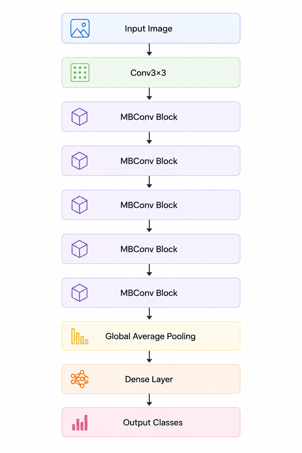
What is an MBConv Block?
EfficientNet is built using:
Mobile Inverted Bottleneck Convolution (MBConv)
Originally introduced in MobileNetV2.
An MBConv block contains:
   Input
     │
     ▼
1×1 Expansion Conv
     │
     ▼
Depthwise Convolution
     │
     ▼
Squeeze-and-Excitation
     │
     ▼
1×1 Projection Conv
     │
     ▼
   Output
Benefits:
- Fewer parameters
- Faster inference
- Better accuracy
Squeeze-and-Excitation (SE) Module
EfficientNet also uses:
Channel Attention
The network learns:
Which channels are important?Example:
For a Husky image:
- Fur texture channel → important
- Background channel → less important
The SE module automatically increases useful channels and suppresses irrelevant ones.
This improves feature quality significantly.
EfficientNet Variants
EfficientNet comes in multiple sizes.
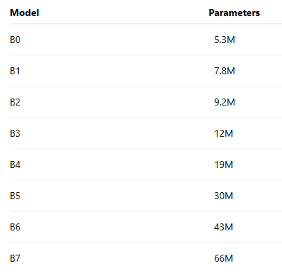
As we move from B0 to B7:
- Depth increases
- Width increases
- Resolution increases
using compound scaling.
Understanding Feature Learning
Let’s classify a German Shepherd.
Early Layers
Learn:
- Edges
- Corners
- Simple textures
////
----
|||||
Middle Layers
Learn:
- Eyes
- Ears
- Fur patterns
Deep Layers
Learn:
German Shepherd Facerather than individual edges.
This hierarchical learning enables accurate classification.
Why EfficientNet Became Popular
Compared to older CNNs:

EfficientNet achieves an outstanding balance between:
- Accuracy
- Speed
- Memory usage
Transfer Learning with EfficientNet
Most real-world projects use pretrained EfficientNet.
Advantages:
- Faster training
- Less data required
- Better performance
Instead of learning from scratch, the model starts with knowledge from ImageNet’s millions of images.
Python Example Using TensorFlow
Load EfficientNetB0
# Import EfficientNetB0 model from Keras applications (pretrained CNN architecture)
from tensorflow.keras.applications import EfficientNetB0

# Load EfficientNetB0 pretrained on ImageNet dataset
# weights='imagenet' → uses learned weights from ImageNet (transfer learning)
# include_top=False → removes the final classification layer (we add our own head)
# input_shape=(224, 224, 3) → expects 224x224 RGB images as input
base_model = EfficientNetB0(
    weights='imagenet',
    include_top=False,
    input_shape=(224, 224, 3)
)
Freeze Pretrained Layers
# Freeze the pretrained EfficientNetB0 base model
# This prevents its weights from being updated during training
# Useful in transfer learning to retain learned ImageNet features
# and train only the custom classification head on top
base_model.trainable = False
Build Classification Model
# Import necessary Keras modules for building the neural network
from tensorflow.keras import layers
from tensorflow.keras import models

# Build a Sequential model by stacking layers on top of the pretrained EfficientNetB0 base
model = models.Sequential([
    base_model,  # Pretrained EfficientNetB0 feature extractor (frozen if base_model.trainable = False)

    # Global Average Pooling reduces spatial dimensions (H x W) into a single vector per feature map
    layers.GlobalAveragePooling2D(),

    # Dropout layer to reduce overfitting by randomly deactivating 30% of neurons during training
    layers.Dropout(0.3),

    # Fully connected dense layer to learn higher-level patterns from extracted features
    layers.Dense(128, activation='relu'),

    # Output layer for 3-class classification using softmax activation
    # Produces probability distribution across the 3 classes
    layers.Dense(3, activation='softmax')
])
Compile Model
# Compile the model by defining how it will learn and be evaluated during training

model.compile(
    optimizer='adam',
    # Adam optimizer: adaptive learning rate optimizer that combines momentum + RMSprop
    # Works well for most deep learning classification problems

    loss='categorical_crossentropy',
    # Loss function used for multi-class classification when labels are one-hot encoded
    # Measures how far predicted probabilities are from true class distribution

    metrics=['accuracy']
    # Evaluation metric to track during training and validation
    # Accuracy = percentage of correctly predicted samples
)
Train
# Train the model using the training dataset and validate on validation dataset

history = model.fit(
    train_dataset,
    # Training data pipeline (input images + labels)

    validation_data=val_dataset,
    # Validation data used to monitor model performance on unseen data during training

    epochs=10
    # Number of complete passes through the entire training dataset
    # Each epoch updates model weights based on backpropagation
)
Example Predictions
Suppose the model sees these images.

The pretrained EfficientNet backbone already understands general visual concepts, making transfer learning highly effective.
When Should You Use EfficientNet?
EfficientNet is an excellent choice when:
✅ High accuracy is required
✅ GPU memory is limited
✅ Dataset size is moderate
✅ Transfer learning is desired
Examples:
- Medical imaging
- Wildlife monitoring
- Industrial inspection
- Dog breed classification
- Agricultural AI
EfficientNet vs Previous Models
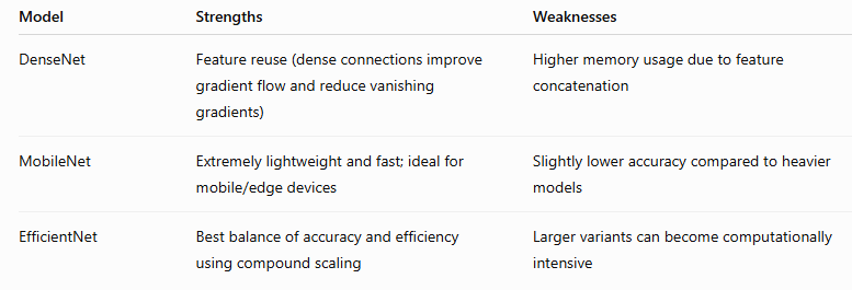
A Quick Reference Guide

Image created by author using AI guidance
Conclusion
EfficientNet revolutionized CNN design by introducing Compound Scaling, a smarter way to increase model capacity. Instead of simply making networks deeper or wider, EfficientNet balances depth, width, and image resolution simultaneously.
The result is a family of models that delivers exceptional accuracy while remaining computationally efficient.
For many computer vision projects, EfficientNet remains one of the strongest choices for transfer learning, offering an ideal combination of performance, speed, and resource efficiency.
References
- EfficientNet: Rethinking Model Scaling for Convolutional Neural Networks https://arxiv.org/abs/1905.11946
- TensorFlow EfficientNet Documentation https://www.tensorflow.org/api_docs/python/tf/keras/applications/efficientnet
- Google Research Blog — EfficientNet https://research.google/blog/efficientnet-improving-accuracy-and-efficiency-through-automl-and-model-scaling/
- Keras EfficientNet API Documentation https://keras.io/api/applications/efficientnet
A Message from AI Mind

Thanks for being a part of our community! Before you go:
- 👏 Clap for the story and follow the author 👉
- 📰 View more content in the AI Mind Publication
- 🧠 Improve your AI prompts effortlessly and FREE
- 🧰 Discover Intuitive AI Tools
메타데이터
- post_id
- e6f11856e4eb
- slug
- a-practical-guide-to-efficientnet-with-python-examples-e6f11856e4eb
- url
- https://pub.aimind.so/a-practical-guide-to-efficientnet-with-python-examples-e6f11856e4eb
- canonical_url
- https://pub.aimind.so/a-practical-guide-to-efficientnet-with-python-examples-e6f11856e4eb
- author_url
- https://medium.com/@sabitha.manoj0891
- status
- ok
- fetched_at
- 2026-07-09 13:13:48