Build a GAN part 2: StyleGAN vs Glow

In this second part, we’ll walk through StyleGAN, then dive into OpenAI’s Glow model.

But first, here are a few things to know (you can skip this part):

• The goal of the generator is not to produce a valid image from every possible latent z, but to do so on average across all z
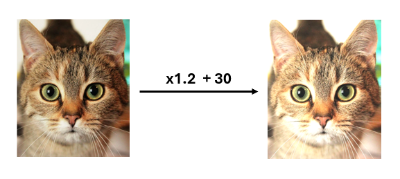
• linear transformation of images preserves the features:

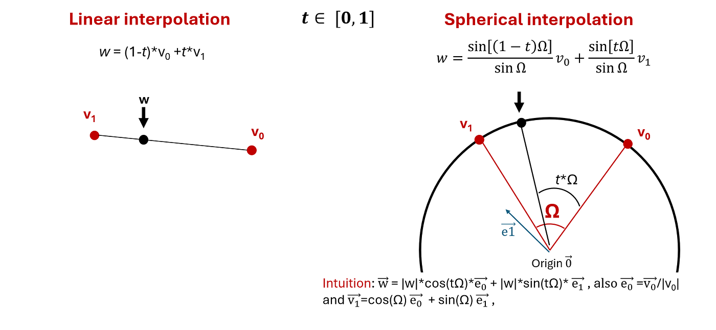
• linear interpolation vs spherical interpolation:

• important concept about the gaussian:

a 2D gaussian distribution (0,1) looks like this :

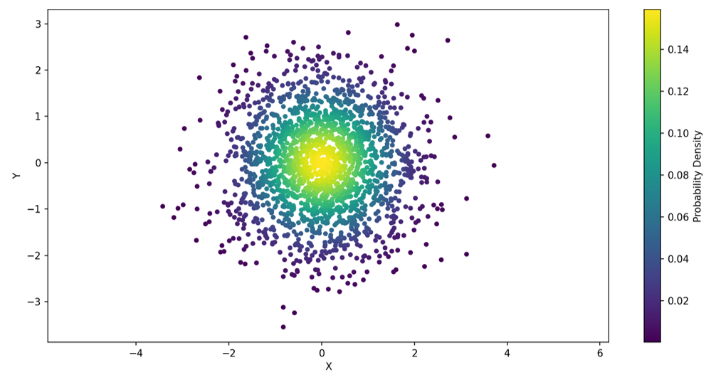
notice that the probability to draw points from an external ring far from the center is bigger than drawing points near the center:

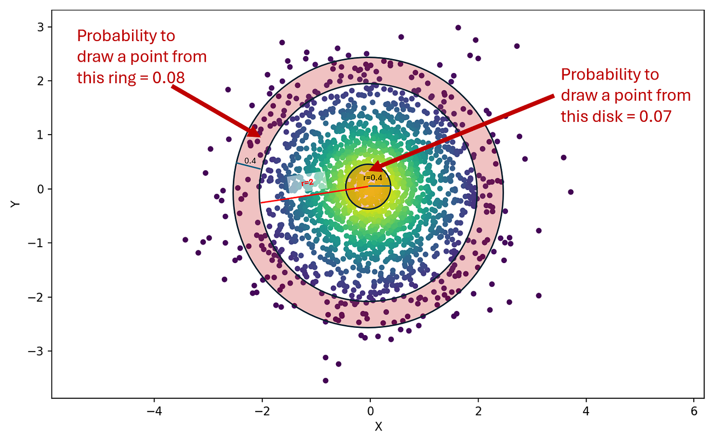
and this is even more visible for bigger dimensions..for an N dimensional standard gaussian, almost every single point you draw will land exactly at a distance sqrt(N) from the center.

• change of variable in a probability density function:

suppose we have x ∈ ℝ and g(x) a bijective and continuous function from ℝ to ℝ. Then g is monotonic. Suppose we define y as y = g(x). Now if we take a segment [a,b] in the X-space, and we calculate its equivalent in the Y-space: a’ = g(a) and b’ = g(b), then every point x in [a,b] will have its image g(x) lying in [a’,b’], and every point in [a’,b’] will have its preimage g⁻¹(y) in [a,b] , because g is bijective and monotonic.

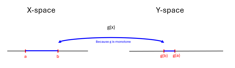
so P(x ∈ [a,b]) = P(y ∈ [a’,b’]) because x ∈ [a,b] ⟺ y ∈ [min(a′,b′),max(a′,b′)]. Now if instead of a segment [a,b] we take a very small segment [x, x+dx], then

and therefore:

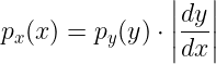
Now if x is multidimensional, we will not have a segment [a,b] but a volume V. The probability that x belongs to that volume is P(x ∈ V). If we choose a very tiny volume, it becomes: pₓ(x)·dVₓ = p_y(y)·dVy (same reasoning as before).

In the 1D case, dy was the transformation of dx and it was a segment. dVₓ is a tiny cube of volume dx₁·dx₂·dx₃·… and dVy is the transformation of that cube into the Y-space , and it is not necessarily a cube; think of it as a distorted cube. A distorted cube is also called a parallelepiped..

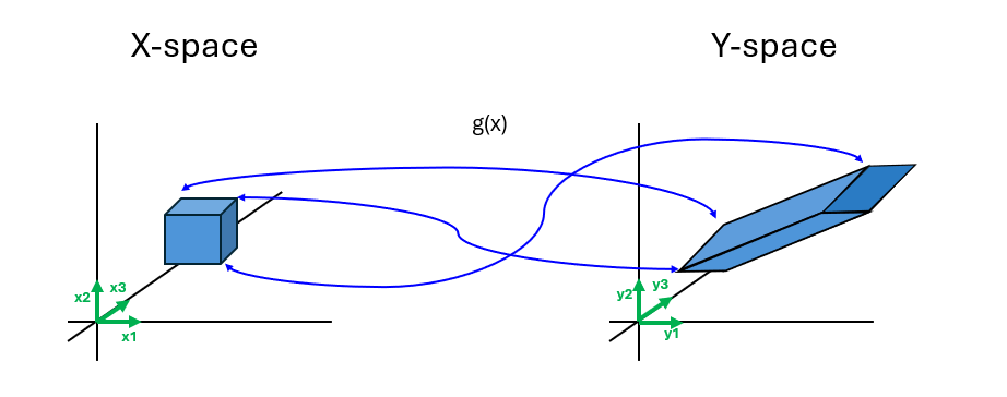
if g is not affine, in macroscopic scale, the volume in Y may not be a parallelepiped. But in the infinitesimally small scale, g behave like an affine function

And if you recall your linear algebra classes, the volume of a parallelepiped is the absolute value of the determinant of the matrix having the coordinates of each edge vector of the parallelepiped as its columns. So we can write our identity as:

where M is the matrix whose columns are the edge vectors of the parallelepiped. We now need to find those vectors.

Given that Y = g(X), dVx is constructed by moving each dimension of X a little bit. For example, a small step of length dx₁ along x₁ (the first dimension of X) corresponds to a step of direction (∂y₁/∂x₁, ∂y₂/∂x₁, …)·dx₁ in Y-space. The vector (∂y₁/∂x₁, ∂y₂/∂x₁, …) captures by how much dx₁ is multiplied in Y-space when taking a step of length dx₁ in the x₁ direction in X-space. The full vector, including the dx₁ multiplier is the first edge vector of the parallelepiped. Doing the same for all dimensions of X and arranging each resulting vector as a column of a matrix (omitting the dx multipliers) , we obtain:

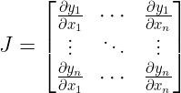
that’s the jacobian of g().

Because we can factor those dx multipliers out of the absolute determinant, our identity becomes

this gives : pₓ(x)=p_y(y)|det(dY/dX)| , and now if you have a proability density function pₓ(x), you can rewrite it as p_y(y)|det(dY/dX)| when the function g is monotone.

StyleGAN:

The problem with traditional GANs is this: suppose our dataset of faces contains no long-haired men. The GAN might still generate a picture of a long-haired man, because the latent z could have a direction corresponding to hair length (since women have various hair lengths and the generator is continuous) and another for masculinity. So there are some latent z that produce long-haired men, and we don’t want that! Because these images fall outside the real data distribution, the discriminator easily flags them as fake (0). So the distribution that generates z should not produce vectors that make this kind of pictures (that’s one of the problems StyleGAN solves).

The discriminator is the same as the ProGAN discriminator we saw in the previous part. Only the generator changes, and here is the generator architecture:

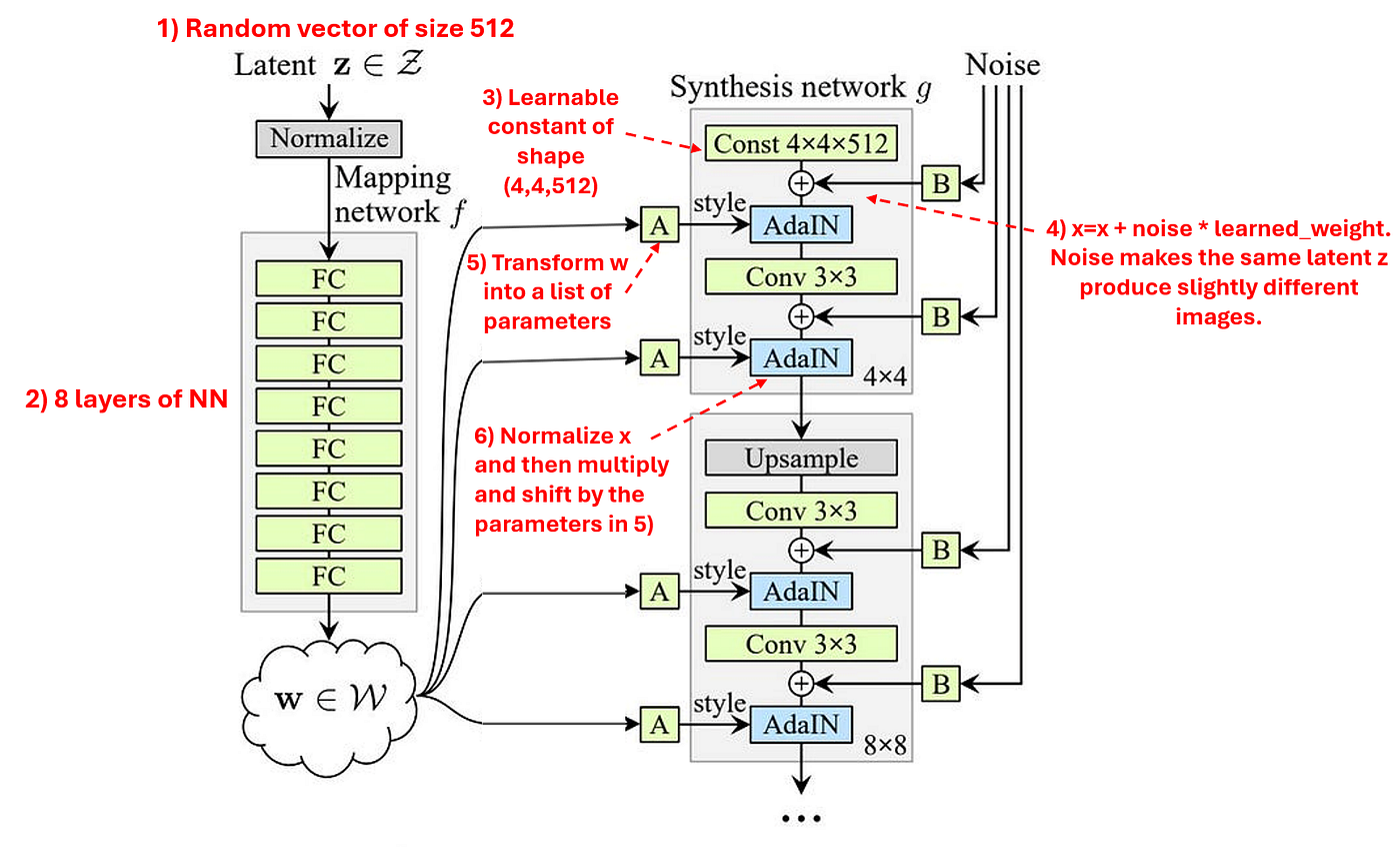
1. generate z using a normal distribution. the shape of z is (N,512)
2. To generate an image, the first step is to pass the random vector z through 8 MLP layers. But why? Simply because learning to map a Gaussian distribution to the real distribution of human faces requires a deeper network. And to make that network bigger, you can either add more convolutions (bad idea!) or stack some linear layers (which is exactly what the authors chose). As a result, the distribution of the latent w is no longer Gaussian; instead, it becomes the optimal probability distribution of latents that helps the generator produce high-quality images. Rare or forbidden feature combinations are therefore naturally avoided. So in StyleGAN, we’re not just learning to generate images through gradient descent, we’re also learning a better representation of the latent space that the generator operates on
3. we feed the generator with a trainable constant of shape (N,512,4,4).

x = tf.get_variable(
 'const', #variable name
 shape=[1, nf(1), 4, 4],
 initializer=tf.initializers.ones()
) #x is trainable

It is the starting point of the 4x4 resolution images (containing 512 feature maps).

4. we just add noise with a learnable weight

5 & 6) Here is an illustration of what happens at the [A] and the [AdaIN] (code) steps:

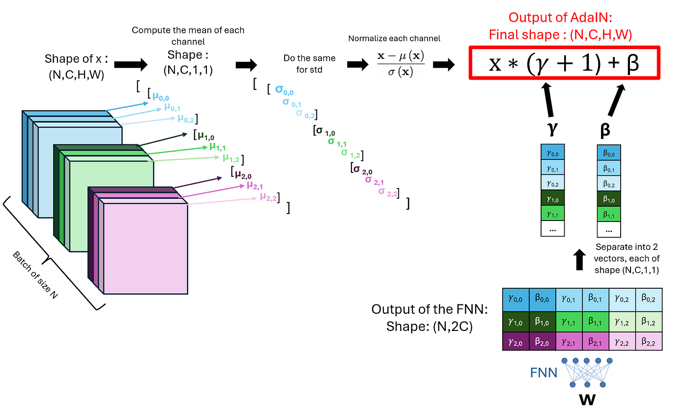
Essentially, the latent w emphasizes or suppresses certain convolutional filter outputs to produce the best images possible. At the early 4×4 generator stage, it controls high-level features such as head shape and skin color etc .., then at late stage (ex : 64x64), it shifts its influence toward finer details like the eyes and nose. So after training, we end up with a latent vector w where different elements control different aspects of the generated output: some influence specific feature maps corresponding to high-level structure, while others govern low-level details.

At the end, after training, the vector W ends up being disentangled. It’s hard to say exactly why the mapping network produces disentangled latents, but I think the intuition is that for a convolutional NN, generating a valid image from a disentangled vector is easier. The loss function is kinda smoother, whereas when the vector is entangled, even a tiny change can result in an invalid image, making the loss landscape rougher and requiring more training steps to reach the optimum.

Here is how the authors proceed to measure that distanglement:

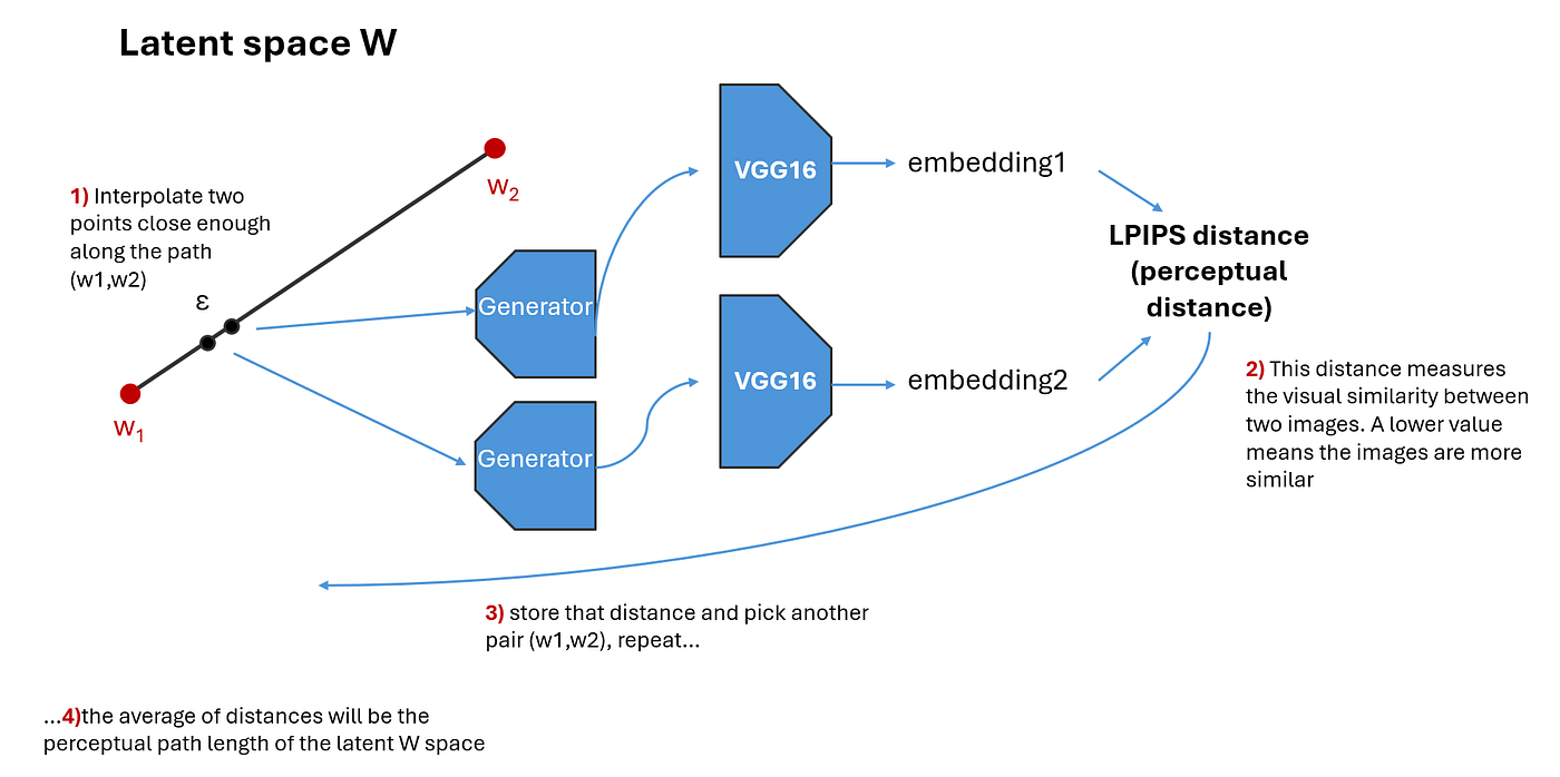
They performed the same analysis on the latent space Z of a traditional GAN. However, for interpolation in Z, they used spherical interpolation rather than linear, because in high dimensions, samples tend to concentrate on a thin spherical shell at radius approximately sqrt(d). Linear interpolation between two samples moves through the interior of the sphere, where points have much lower probability under the Gaussian. Spherical interpolation keeps the interpolation path within the typical high-probability region of the distribution.

They then compared the two perceptual path lengths, and found that the perceptual path length of the latent space W in a StyleGAN generator (with random noise inputs) is lower than that of the latent space Z in traditional generators.

In the official StyleGAN code, you will see what they call : the truncation trick. The goal of this is to avoid the generator to generate image that are not very represented in the training set. Because it will usually generate garbage. To achieve this, when generating the latent vector w, we bring it closer to the average w: w̄, which represents the latent of the most common facial features in the training data. We therefore transform w into w’:

ψ is set to 0.7

The dataset used to train styleGAN contains 70000 images (FFHQ dataset). I implemented a basic verison of StyleGAN and train it on a very small dataset ( 7000 images) , but the results were no better than the previous ones.

Glow

Let’s now dive into another way to generate images: Glow. Instead of a Generator and Discriminator, we train a model f that maps an image x to a latent variable z, such that z follows a normal distribution and x is a real image given as input. Once the model is trained, we simply use its inverse f⁻¹ to generate a new image from a sampled latent z.

Ideally, the loss function should be minimized when x is a real face image , and maximized otherwise…while also enforcing that z follows a normal distribution. The loss function for a given image x is therefore:

Loss(x, θ) = −log(p_θ(x))

where θ denotes the model’s parameters. The loss is minimal when p_θ approximates the true distribution of images.

What could the expression of p_θ actually look like? A neural network, perhaps? No! because for p_θ to be a valid probability distribution, the sum of p_θ(x) over every possible image in the universe must equal exactly 1, which is impossible to guarantee with a standard NN.

Here is how we can derive the expression of p_θ(x): suppose we have a function g_θ that transforms an image x into a latent noise vector z into an image x, i.e. x= g_θ(z). If g_θ is bijective, we can apply the change of variables formula introduced in the prerequisites, which gives us:

p_θ(x) = p_z(z) · |det(dz/dx)|

A general algorithm should look like this (recall that f is bijective, and therefore invertible):

loss = 0
for every real image x:
  z = f(x) #generate latent z from the image
  loss = -(log(p_z(z)) + |log_determinant(Jf)|) #Jf is the jacobian of f
  gradient descent to update f

p_z is N(0,I). In reality GLOW model does not produce a single latent z from an image..it produces a vector of latents (z₁, z₂, z₃, …, z_L), each representing some features of the image. By the chain rule of probability, P(z) can be written as:

if we reverse the order of variables:

let’s apply this to the algorithm:

loss = 0
for every real image x:
  z1,z2,z3..zL = f(x)
  loss = -(log(p(z1|z2,z3...)) + log(p(z2|z3,z4,..zL)) +....+ log(p_z(zl))+ log_determinant(Jf))
  gradient descent to update f and update the parameters of each p(zi|zi+1,...)

where p(z_L) = N(0, I), but p(zi | z{i+1}, z_{i+2}, …, z_L) are Gaussians N(µ, σ). One could simply concatenate all the z_i and evaluate log p(z) in one shot, but the authors of Glow decided it is better to evaluate each conditional probability p(zi | z{i+1}, …) individually.

We know that if variables a and b follow a normal distribution, the conditional probability p(a|b) is itself a Gaussian whose mean and variance depend on b. Therefore,

can be expressed as

where the parameters µ = g(z{i+1}, z{i+2}, …) and σ = t(z{i+1}, z{i+2}, …))are determined by two learned functions g() and t().

Of course, in practice, we do not use a single function f to produce all the z_i at once, rather, each pass through the network produces a single z_i.

This raises an important question: how can we compute µ = g(z{i+1}, z{i+2}, …) when z{i+1}, z{i+2}, … are not yet available? Well, instead of computing p(zi | z{i+1}, z_{i+2}, …, z_L) directly, we compute p(z_i | a vector that will lead to all subsequent zi). This is justified by a standard result from probability theory: if (v, w) is obtained from u through a bijective transformation, then p(a|u) = p(a|v, w). Since the subsequent latents z{i+1}, z_{i+2}, …, z_L ​ are obtained from x via bijective mappings, meaning x perfectly determines them and vice versa, conditioning on x is entirely equivalent to conditioning on all subsequent z_i.

so the code should look like this:

loss = 0
for every real image x:
  for i in range(L-1):
     x,zi=f(x)
     µ,σ= g(x),t(x) #p(zi|zi+1,zi+2) is the same as p(zi|x) because zi+1, zi+2,zi+3
     #will be calculated from x with bijective operations.
     loss -= log(N(zi, mean=µ, std=σ)) #this calculates : log(p(zi|zi+1))
  x,zL=f(x)
  loss -= log(p(zL))
  loss -= log_determinant(Jf))
  gradient descent to update f() and g() and t()

in reality, internally f will split x in half to create z. let’s write the split operation outside f. Also f is applied several time on x.

loss = 0
for every real image x:
  for i in range(L-1):
     for j in range(K): #f is applied several time on x
       x=f(x)
     zkeep,zi = split(x) #splits the channels in half
     µ,σ= g(zkeep),t(zkeep) #zi+1 will be generated form zkeep
     loss -= log(Nµσ(zi)) 
     x=zkeep
  for j in range(K):
    x =f(x)
  zL = x
  loss -= log(p(zL))
  loss -= log_determinant(Jacobian of all function applied to x))
  gradient descent to update f() and g() and t()

log_det of the jacobian of f1(f2(f3(x))) is

so:

loss = 0
for every real image x:
  for i in range(L-1):
     for j in range(K):
       x,log_det=f(x)
       loss -= log_det
     zkeep,zi = split(x) #splits the channels in half
     µ,σ= g(zkeep),t(zkeep) #zi+1 will be generated form zkeep
     loss -= log(Nµσ(zi)) 
     x=zkeep
  for j in range(K):
    x,log_det =f(x)
    loss -= log_det
  zL = x
  loss -= log(p(zL))
  gradient descent to update f() and g() and t()

The authors also added a squeeze operation to reshape the tensor before applying f(). Also, f is actually what we call a “step_of_flow” it means it is a composition of 3 functions , all bijective and invertible.

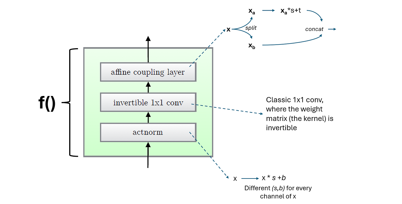
One step of flow

All of these flow step transformations have easily computable log-determinants of their Jacobians. Take ActNorm for example: it performs an element-wise multiplication of the input tensor X by a scale vector s. The Jacobian is simply the matrix dY/dX, and its log-determinant equals H·W·Σlog|s|. To see why, consider flattening both X and Y. The scale vector s has one value per channel: s₁ for the first channel (so the first HW elements of s are s₁) , s₂ for the second, and so on.. For the first HW elements of Y (corresponding to channel 1), we have dYᵢ/dXᵢ = s₁ and dYᵢ/dXⱼ = 0 for i ≠ j, since Yᵢ = Xᵢ · s₁. For the next HW elements (channel 2), dYᵢ/dXᵢ = s₂ and dYᵢ/dXⱼ = 0, and so on for each subsequent channel. This gives a diagnoal matrix whose diagonal consists of HW repetitions of s₁, followed by HW repetitions of s₂, then s₃, etc. The log-determinant of a diagonal matrix is simply the sum of the logs of its diagonal entries, which gives H·W·Σlog|sᵢ|. This is exactly what is returned in log_det when computing x, log_det = f(x).

more details about the Affine coupling layer:

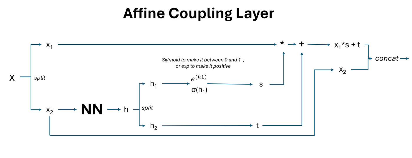
what brilliant about this layer, is that it is invertible even though the NN operation is not. Because when inverting the network, we can compute s and t from the output x2 by simply recomputing NN(x2).

a final algorithm for GLOW would be :

for every real image x:
  x = preprocess(x)
  loss = 0
  final_z = []
  for i in range(L-1):
     x = squeeze(x)
     for _ in range(K):
       x,log_det=step_of_flow(x)
       loss -= log_det
     zkeep,zi = split(x)
     final_z.append(zi)
     µ,σ= generate_parameters(zkeep) 
     loss -= log(N(zi, mean=µ, std =σ )) 
     x=zkeep
  x = squeeze(x)
  for _ in range(K):
    x,log_det =step_of_flow(x)
    loss -= log_det
  zL = x
  final_z.append(zL)
  loss -= log(N(zL))
  gradient descent to update step_of_flow() and generate_parameters()

You can see the GLOW model as :

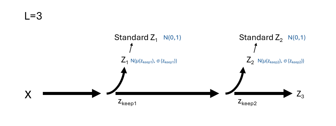
illustration of Glow model. x is the image

Then, once the model is trained, generating an image is very simple: :

1. First, we sample a random vector Z3 from a standard normal distribution, matching the shape of Z3. We then pass it backward through the model:

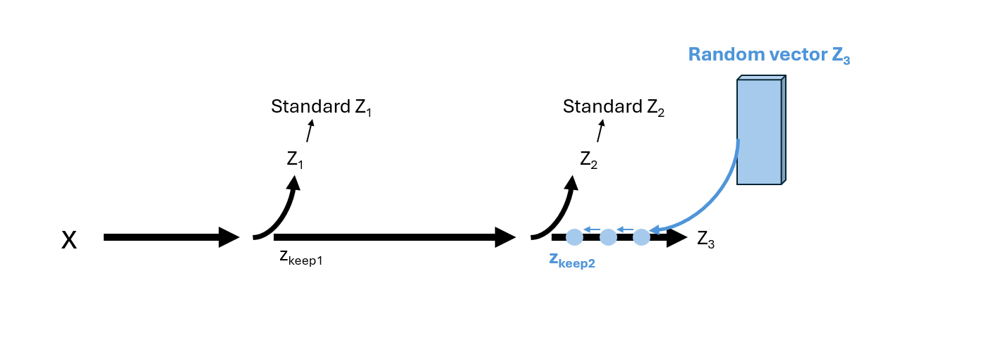
2. Next, we sample a standard random vector Z2 (with the same shape as Z2), from which we can derive Z2, since Z2 ~ N(µ(Zkeep2), σ(Zkeep2)) using the same µ() and σ() functions from training.

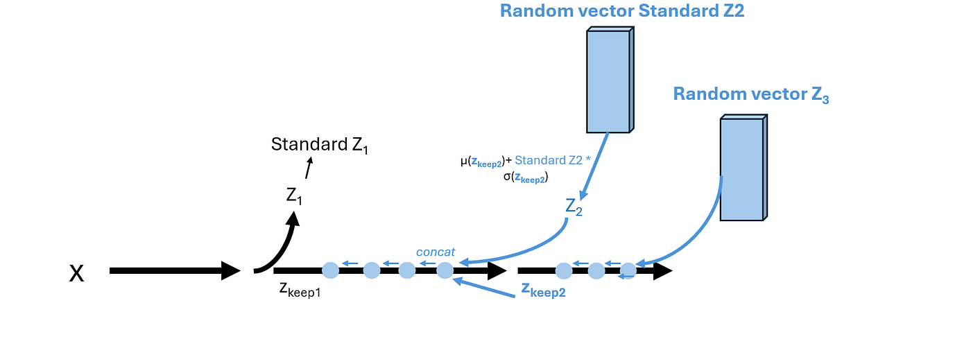
We repeat this process until the image x is fully constructed.

You can find my implementation of a simplified Glow model here: code

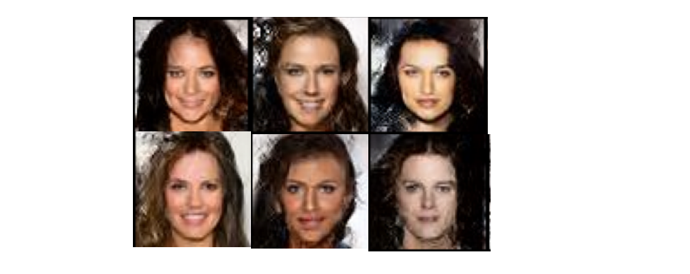
The results are not bad for a toy model, especially given that it was trained for only a few epochs:

That brings us to the end of Part 2. We’ve covered a lot of ground between StyleGAN’s style-based architecture and Glow’s normalizing flows , two very different approaches to the same challenge. If you have questions or spot something worth discussing, the comments section is all yours. In the next article we will see how to generate music with GANs

[embed]Glow: Better reversible generative models We introduce Glow, a reversible generative model which uses invertible 1x1 convolutions. It extends previous work on…openai.com

https://stats.stackexchange.com/questions/239588/derivation-of-change-of-variables-of-a-probability-density-function