The Chain of Failures: How Data Structures Actually Evolved

Why every data structure exists to fix the last one’s mistake

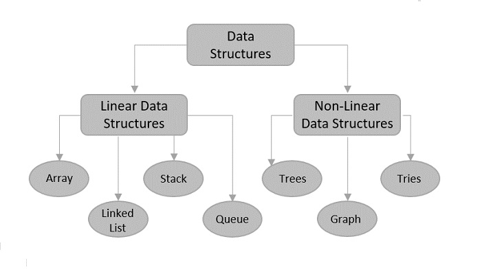
https://www.tutorialspoint.com/data_structures_algorithms/images/data_structures_and_types.jpg

Every data structures textbook is organized as a catalog: here are the tools, here are their big-O characteristics, here is when to use them. However, the catalog framing has one systematic flaw: It transmits solutions without transmitting the failures that produced them. By the time a structure reaches a textbook, the historical contingency is gone and the thing looks like a deliberate design choice rather than the consequence of a specific wall being hit.

An engineer who knows the solution without knowing the failure mode has learned a pattern without developing a judgment. Every data structure was built to address a specific problem. The complexity it introduces is a cost, justified only by the failure mode it exists to solve. If you haven’t hit the failure mode, the simpler structure is not naive, it is correct.

What follows is not a catalog. It is the chain of failures.

1. Arrays: The Baseline

Start with the array because everything else is a reaction to it.

An array is a contiguous block of memory. That contiguity is everything. When you write arr[40000], the CPU computes a single address base_address + 40000 * sizeof(int) and fetches it in one step. This is O(1) random access, and the reason it works is purely physical: RAM is addressable by location, so if you know where something starts and how big each element is, you can find any element without touching any other element.

int arr[5] = {10, 20, 30, 40, 50};
printf("%d\n", arr[2]); // Always one operation, regardless of array size

There is a second, subtler win here that big-O notation does not capture: cache locality. Modern CPUs don’t fetch single bytes, they fetch cache lines of 64 bytes at a time. When you read arr[0], the CPU pulls arr[0] through arr[15] (for 32-bit ints) into L1 cache simultaneously. Sequential array traversal is fast not just in theory but on the physical machine too because you're exploiting that prefetch behavior.

Now here is where the array breaks.

Suppose you have an array of one million sorted integers and you need to insert a new value in the middle. The value’s correct position is index 500,000. Every element from index 500,000 to 999,999 must move one slot to the right to make room. That’s a memmove of 500,000 × 4 bytes, two megabytes of data shuffling in memory. The operation is O(n), and it's O(n) in a brutal, physical way: the CPU is touching half your dataset to perform one logical insertion.

void insert(int* arr, int n, int pos, int val) {
    memmove(&arr[pos + 1], &arr[pos], (n - pos) * sizeof(int));
    arr[pos] = val;
}

This is the failure mode. The array’s performance model is tied to contiguity, and contiguity requires shifting. If you need fast insertion or deletion at arbitrary positions, the array cannot give it to you. That wall is what forces the next structure into existence.

2. Linked Lists: Fixing Insertion

The linked list’s insight is simple: stop enforcing contiguity. Instead of storing elements adjacently in memory, store each element in its own node that carries a pointer to the next one. Nodes can live anywhere in memory because their logical order is encoded in the pointers, not their physical addresses.

typedef struct Node {
    int data;
    struct Node* next;
} Node;

Node* insert_at_head(Node* head, int val) {
    Node* node = malloc(sizeof(Node));
    node->data = val;
    node->next = head;
    return node; // One allocation, two pointer assignments. O(1).
}

Insertion is now O(1) at the head, or O(1) anywhere you already have a pointer to the predecessor. You’re redirecting pointers. The array’s insertion wall is gone.

But the linked list doesn’t eliminate the wall. It moves it.

The array’s strength was contiguity. When you destroy contiguity, you destroy random access. To find element at position k in a linked list, you must start at the head and follow k pointers in sequence. There is no formula for jumping directly to position k, each node’s address is encoded in its predecessor, not derivable from k. Access is O(n).

And here the hidden tax appears from the other direction. Recall the cache line: when you traverse a linked list, each node dereference is a pointer chase to an arbitrary heap address. The CPU cannot predict where the next node lives, so it cannot prefetch it. Every node = node->next is potentially a cache miss, a full trip to main memory, which is 100–200x slower than an L1 hit. A linked list traversal over a million nodes can be dramatically slower in wall-clock time than the O(n) notation suggests compared to an array traversal, because the array version is cache-friendly and the linked list version is not.

The mathematical complexities are identical. The physical runtimes are not. This is the gap.

You have paid for insertion with access speed and cache behavior. This cost is real and cannot be escaped, it is a direct consequence of the freedom from contiguity that solved the insertion problem. The linked list is correct when your problem requires frequent arbitrary insertion and does not require frequent arbitrary access. If you need both, you are not done yet.

3. Stacks and Queues: When the Constraint Is the Point

Stacks and queues are not new data structures in any deep sense. A stack is a linked list where you only ever touch one end. A queue is a linked list where you add to one end and remove from the other. The data structure is the same; the interface is deliberately restricted.

Node* push(Node* top, int val) {
    return insert_at_head(top, val);
}

int pop(Node** top) {
    Node* temp = *top;
    int val = temp->data;
    *top = temp->next;
    free(temp);
    return val; // O(1): always touching the head
}
typedef struct {
    Node *front, *rear;
} Queue;
void enqueue(Queue* q, int val) {
    Node* node = malloc(sizeof(Node));
    node->data = val;
    node->next = NULL;
    if (!q->rear) { q->front = q->rear = node; return; }
    q->rear->next = node;
    q->rear = node; // O(1) because we hold a pointer to the tail
}

The tail pointer in the queue deserves attention, because it is the difference between O(1) and O(n) enqueue, and it is not obvious from the abstract definition. The definition says “add to the rear.” The implementation question is how you find the rear without traversal. The answer is: you maintain a second pointer and update it on every enqueue. The math says O(1); the implementation earns that O(1) by carrying extra state.

The reason stacks and queues are useful despite inheriting the linked list’s access limitations is that they eliminate the problem entirely through interface restriction. If your algorithm only ever touches the most recent or oldest element, then the O(n) random access cost simply does not arise. You have designed around it by choosing a problem that doesn’t have it.

This is the key insight, and it is worth stating explicitly: the correct response to a data structure’s failure mode is not always a more complex structure. Sometimes it is a constraint that makes the failure mode irrelevant. Stacks and queues are strictly less capable than linked lists, and that restriction is precisely what makes them correct for LIFO and FIFO problems. The call stack, browser history, task scheduling, all of these have natural ordering semantics that eliminate the need for random access.

4. Hash Maps: Eliminating Search Entirely

Suppose you need to associate arbitrary keys with values and retrieve them in O(1). No traversal, no ordering, just: given this key, give me this value, fast. The array can do this if your keys are dense integers, you index directly. But what if your keys are strings? Or GUIDs? Or user-defined objects? Arrays over arbitrary key spaces are not possible. You need a new idea.

The hash map’s insight is to convert arbitrary keys into array indices. If you can turn “username” or 0xDEADBEEF into a number in the range [0, TABLE_SIZE), you can store and retrieve by key in O(1), using an array for the storage. The failure mode being addressed is: I have arbitrary keys and I need constant-time lookup.

#define TABLE_SIZE 64

typedef struct Entry {
    int key;
    int value;
    struct Entry* next; // For collision chaining
} Entry;
Entry* table[TABLE_SIZE];
unsigned int hash(int key) {
    return (unsigned int)key % TABLE_SIZE;
}
void put(int key, int value) {
    unsigned int idx = hash(key);
    Entry* e = malloc(sizeof(Entry));
    e->key = key; e->value = value;
    e->next = table[idx];
    table[idx] = e;
}
int get(int key) {
    unsigned int idx = hash(key);
    Entry* e = table[idx];
    while (e) {
        if (e->key == key) return e->value;
        e = e->next;
    }
    return -1;
}

The O(1) claim requires careful examination. The get function has a while loop. How is this O(1)?

It is O(1) on average, assuming a good hash function and a low load factor. Both assumptions are mathematical conditions, and both can fail in practice.

A bad hash function clusters keys into a small number of buckets. If hash(key) returns the same index for every key, all entries pile into one chain and get degrades to O(n). The hash function key % TABLE_SIZE is particularly vulnerable if keys are multiples of TABLE_SIZE because they all hash to zero.

The load factor α = n / TABLE_SIZE controls the expected chain length. When α is high, chains are long and lookup is slow. Most real implementations resize the table when α exceeds a threshold (typically 0.75), rehashing all existing keys into a larger array. That resize is O(n), but infrequent enough that the amortized per-operation cost stays O(1).

This is a deeper gap than the linked list’s cache miss problem, because it is about the conditions under which the mathematical proof holds. The implementation must actively maintain those conditions, or the guarantee evaporates. You have O(1) lookup, but only if you choose a good hash function, monitor the load factor, and resize proactively. Let any of those slip and the issue reappears.

The new wall the hash map builds: ordering is gone. A hash map does not preserve insertion order and provides no efficient way to find “the smallest key” or “all keys in some range.” The scrambling that distributes keys evenly is precisely what destroys their order. If you need ordered keys, the hash map is the wrong tool.

5. Binary Search Trees: Ordering the Search

The wall the hash map builds is the loss of ordering. A binary search tree exists to address exactly that failure mode: I need both fast lookup and ordered traversal.

A BST stores elements in a tree with one invariant: for every node, all values in the left subtree are smaller, and all values in the right subtree are larger. That invariant enables binary search, at each node, compare your target to the current value and follow the appropriate branch. You are eliminating half the remaining candidates at every step.

typedef struct BSTNode {
    int data;
    struct BSTNode *left, *right;
} BSTNode;

BSTNode* insert(BSTNode* root, int val) {
    if (!root) {
        BSTNode* node = malloc(sizeof(BSTNode));
        node->data = val;
        node->left = node->right = NULL;
        return node;
    }
    if (val < root->data)      root->left  = insert(root->left, val);
    else if (val > root->data) root->right = insert(root->right, val);
    return root;
}
BSTNode* search(BSTNode* root, int val) {
    if (!root || root->data == val) return root;
    return val < root->data
        ? search(root->left, val)
        : search(root->right, val);
}

If the tree has height h, search takes O(h). For a balanced tree with n nodes, h = ⌊log₂ n⌋ and search is O(log n). For a million nodes, that’s 20 comparisons.

Here is the failure mode, and it is a subtle one: the O(log n) guarantee requires the tree to be balanced, but the naive insertion algorithm does not ensure balance.

Insert the values 1, 2, 3, 4, 5 in order. Each new value is larger than all existing ones, so it always goes right. The tree degenerates into a right-skewed linked list:

1
 \
  2
   \
    3
     \
      4
       \
        5

Height is n, not log n. Search is O(n). The code is correct but its performance guarantee has collapsed because the guarantee was conditional on balance that insertion order can silently destroy.

The fix of self-balancing trees like AVL trees or red-black trees adds rotation operations that restructure the tree after insertions to maintain balance. The implementation is substantially more complex: an AVL tree’s insert is perhaps five times longer than the one above, because it must compute balance factors and perform rotations. The O(log n) guarantee becomes unconditional, but you pay in implementation complexity and constant factors.

The balanced BST required decades of research to achieve correctly. AVL trees arrived in 1962. Red-black trees in 1978. These were not obvious refinements. They were genuine innovations, and each one was motivated by the specific failure mode of the naive BST under adversarial or sorted input.

6. Heaps: When You Only Need the Extremum

The specific failure mode addressed here is: I need to repeatedly extract the maximum (or minimum) from a dynamically changing set, as efficiently as possible.

A heap is a tree where every node is greater than or equal to its children (a max-heap). The root is always the maximum. Insert and extract-max are both O(log n). But the heap gives up something the BST provided: arbitrary ordered search. You cannot find an arbitrary element in a heap without a full scan. It is fast at exactly what priority queues need, and offers nothing else.

int heap[MAX_SIZE];
int size = 0;

// For node at index i:
// Parent:       (i - 1) / 2
// Left child:   2*i + 1
// Right child:  2*i + 2
void heapify_up(int idx) {
    while (idx > 0) {
        int parent = (idx - 1) / 2;
        if (heap[idx] > heap[parent]) {
            int tmp = heap[idx];
            heap[idx] = heap[parent];
            heap[parent] = tmp;
            idx = parent;
        } else break;
    }
}
void insert(int val) {
    heap[size] = val;
    heapify_up(size++);
}
int extract_max() {
    int max = heap[0];
    heap[0] = heap[--size];
    heapify_down(0);
    return max;
}

The heap is stored as a flat array. No pointers. No dynamic allocation per node. The tree structure is encoded arithmetically in array indices. This is not obvious from the abstract definition of a heap, which describes a tree. The array encoding is an implementation insight earned by someone who noticed that the tree is always complete since every level is full except possibly the last which means the parent-child relationships can be computed from index arithmetic rather than stored as pointers. The result is better cache performance than a pointer-based tree and no per-node allocation overhead.

The O(log n) for both operations is directly visible in the code. heapify_up runs at most ⌊log₂ n⌋ times because each iteration moves one level up in the tree, and the tree's height is ⌊log₂ n⌋. The logarithm is the number of times you can halve an integer before reaching zero, which is exactly what the index arithmetic is doing.

One subtlety worth examining: extract_max moves the last array element to position 0 before calling heapify_down. Why? Because removing the root and leaving a hole breaks the tree structure. Moving the last element to the root is the only O(1) operation that fills the hole while keeping the array contiguous. The heap property is then violated at the root and heapify_down repairs it in O(log n). The algorithm works by deliberately violating and then restoring the invariant in a controlled way.

The heap is the clearest example in the chain of a structure that is strictly less capable than its predecessor by design. You cannot do everything a BST does with a heap.

7. Graphs: The Structure That Contains All the Others

Every structure so far is a special case of a graph. An array is a graph where each node connects only to its sequential neighbor. A tree is an acyclic connected graph. A BST is a tree with an ordering invariant. Graphs are the general case: a set of vertices connected by edges, with no restrictions on connectivity, direction, or weight.

The interesting question is not what a graph is, it is how to store one, because there is no single answer. The right representation depends entirely on the graph’s density, and the tradeoff is direct.

Adjacency matrix:

int matrix[MAX_V][MAX_V] = {0};
void add_edge(int u, int v) {
    matrix[u][v] = 1;
    matrix[v][u] = 1;
}
int has_edge(int u, int v) {
    return matrix[u][v]; // O(1)
}

has_edge is O(1). But the matrix requires O(V²) space regardless of the number of edges. For a social network with a million users where the average person has 200 friends, you are allocating space for a trillion edge slots to store 200 million actual edges. The matrix is 99.98% empty.

Adjacency list:

typedef struct AdjNode {
    int vertex;
    struct AdjNode* next;
} AdjNode;

AdjNode* adj[MAX_V];
void add_edge(int u, int v) {
    AdjNode* node = malloc(sizeof(AdjNode));
    node->vertex = v;
    node->next = adj[u];
    adj[u] = node;
}
int has_edge(int u, int v) {
    AdjNode* node = adj[u];
    while (node) {
        if (node->vertex == v) return 1;
        node = node->next;
    }
    return 0; // O(degree(u))
}

has_edge is now O(degree(u)). Space usage is O(V + E), proportional to what you actually store.

Neither representation is better. Each is correct for a specific problem shape. Dense graphs with frequent edge queries: matrix. Sparse graphs with frequent neighbor iteration: adjacency list. The abstract structure is identical. The performance profiles are opposed.

Conclusion

The chain is not a ladder of sophistication. It is a sequence of specific failures and the structures they forced into existence. Arrays break on insertion. Linked lists fix that and break random access. Stacks and queues don’t solve the access problem, they pick problems that don’t have it. Hash maps eliminate search and lose ordering. BSTs restore ordering and collapse to O(n) on sorted input until decades of research made the balance guarantee unconditional. Heaps give up arbitrary access to earn a cache-friendly priority queue. Graphs contain all of the above and have two opposed implementations depending on whether your data is dense or sparse.

Every step is a negotiation. The failure mode of the previous structure is addressed; a new one is introduced.

The engineer who has internalized the failures looks at a problem and sees which wall they will hit. The engineer who has only internalized the catalog reaches for the most complex structure they’ve memorized, because complexity is the only axis the catalog gives them.