LoRA & QLoRA Mastery: The Beginner-to-Advanced Guide to Efficient LLM Fine-Tuning

Understand the intuition behind LoRA and QLoRA, learn the math without getting lost in equations, and fine-tune LLMs efficiently using Hugging Face, PEFT, and real-world code examples.

Hello, If you’ve ever wanted to fine-tune a Large Language Model but were held back by massive GPU requirements or expensive training costs, LoRA (Low-Rank Adaptation) is the technique you need to know. It has become one of the most widely adopted methods for efficiently adapting large language models with just a fraction of the parameters.

In this guide, we’ll dive deep into what LoRA is, why it works, the mathematics behind it, how to train and use it in practice, and when you should (or shouldn’t) choose it. Whether you’re a beginner or an experienced ML engineer, this guide will help you build a solid understanding of LoRA from first principles to real-world implementation.

Why Do We Need LoRA?

Before we understand what LoRA is, we first need to understand why it was introduced in the first place. Like every major innovation in machine learning, LoRA exists to solve a real problem.

We’ll start by exploring what fine-tuning is, how full fine-tuning works, and why it becomes computationally expensive for today’s large language models. Once we understand these limitations, we’ll see how LoRA provides an elegant and highly efficient solution to overcome them.

Step 0: What is Finetuning

You take a model that’s already been trained on a massive general dataset (this is “pretraining”, it already knows grammar, facts, reasoning patterns), and you continue training it on a smaller, task-specific dataset so it gets good at your specific job (e.g., medical Q&A, customer support tone, code generation in your style).

Step 1: The Original Way: Full Fine-Tuning

You update every single weight in the model. Nothing is frozen. The model recalculates gradients for all 7 billion parameters and adjusts all of them during training.

When you just download and run (inference only) a 7B model, memory needs are simple:

• Weights stored in 16-bit precision (fp16/bf16): 7B params × 2 bytes = ~14 GB

That’s it for inference. You load it, run it, done.

But the moment you want to train it (full fine-tuning), you need to store a lot more, because of how backpropagation + the Adam optimizer work:

Imagine you download a large model like:

• LLaMA
• Qwen
• GPT-like model

Let’s say:

• Model size = 7 billion parameters
• Stored in FP32 ( if you want to learn more about Quantization, you can read here)
• That’s ~28GB memory

If you want to teach it a new task (like medical Q&A):

You do:

model = AutoModelForCausalLM.from_pretrained("model")
trainer.train()

What happens?

1.) All weights update 2.) Gradients stored for all parameters 3.) Optimizer states stored

Memory needed:

• Model weights (The model itself) : ~28GB
• Gradients (One gradient per weight, computed every backward pass) : ~28GB
• Adam optimizer states (2 extra copies): ~28*2 = 56GB

Total: ~112 GB, just to hold the state, before you’ve even fed it a single batch of training data. Add activations (intermediate outputs stored for backprop) and that climbs further depending on batch size and sequence length.

That’s why full fine-tuning a 7B model basically requires multiple 80GB GPUs (A100/H100) with the load split across them, it physically doesn’t fit on one consumer GPU.

This is exactly the problem LoRA solves

Step2: The Core Problem

Most of the model already knows language.

You don’t need to change all 7B parameters to:

• Make it medical
• Make it legal

You only need small adjustments.

That leads to: PEFT — Parameter Efficient Fine Tuning

PEFT is not one method. It’s a category.

**It means: **Fine-tune only a small number of parameters instead of the whole model.

Examples of PEFT:

1.) Adapters 2.) Prefix tuning 3.) Prompt tuning 4.) LoRA 5.) IA3 6.) QLoRA

So: ✔ Base model frozen ✔ Add small trainable parameters ✔ Only those get updated

Memory becomes small.

Today, we gonna discuss only about LoRA.

LoRA (Low Rank Adaptation): It’s a way to fine-tune a huge pretrained model (like Llama or GPT) without touching most of its original weights.

What LoRA Actually Does ?

In transformers, most learning happens inside: Linear layers

Example: Y = W × X

Where:

• W is huge (like 4096 × 4096)
• That’s millions of parameters

LoRA says:

Instead of updating W, Keep W frozen, Add a small low-rank matrix update.

Mathematically:

W_new = W + ΔW

LoRA approximates:

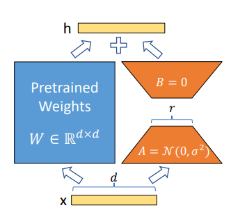
ΔW = A × B

Where:

• A = (d × r)
• B = (r × d)
• r = small rank (like 8 or 16)

So instead of updating millions of parameters:

You update:

2 × d × r

Wait wait wait, its going too technical, lets stop here and see what is happening.

What is ΔW? How do we get it ? what are the values inside A and B ?

Too Many Questions ? Good. Asking these questions is the first step to understanding the concept.

Lets understand:

A transformer linear layer: Y= W * X

W= pretrained weight X = input Y= Output

1. ) Normal Full Fine tuning:

We start with:

W0= W_original

After training:

W= W_trained

Here we directly update W. So, in Full Fine-tuning, there is no separate ΔW stored anywhere. We just modify W directly.

Okay, now lets see how ΔW comes into the picture in LoRA.

LoRA says:

Instead of updating W, Keep W frozen, Add a small low-rank matrix update.

Mathematically:

W_new = W + ΔW

Here, we are not updating W, just like Full Finetuning, we are just updating ΔW.

Now you must be thinking, How can we separate ΔW and W, right ?

Lets understand this:

Imagine: 

W_original = 10

After training:

W_trained = 13

Then:

ΔW = 3 ( 13-10 )

So:

W_new = 10 (W_original) + 3 (ΔW) = 13
W_new = W + ΔW

W is just the base. ΔW is the change.

Okay, I got how we divided ΔW and W. But what is exactly ΔW ? and how it is benefitting LoRA ?

So, Instead of learning a full matrix ΔW (same size as W), we approximate it using low-rank factorization.

LoRA assumes:

ΔW = A × B

Where:

• A = (d × r)
• B = (r × d)
• r = small rank (like 8 or 16)
• So instead of learning a full d × d update (which would be 4096 × 4096 = ~16.7M numbers), you learn it through a narrow r-dimensional bottleneck. If r = 8, you're learning:

A: 4096 × 8 = 32,768 params
B: 8 × 4096 = 32,768 params
Total: 65,536 params

That’s ~250x fewer parameters than the full matrix.

The intuition: the change needed to adapt a pretrained model to a new task usually doesn’t need the full d-dimensional richness, it lives in a much smaller subspace. r is how big you let that subspace be.

Now, what is this d, r, and how are we going to decide the value of r ?

d is the dimension of the original weight matrix you're adapting. If you're targeting the attention projection in Llama 7B, that weight matrix might be something like d × d = 4096 × 4096. So d is just "how big is the layer," and it's fixed, it comes from the model's architecture, you don't choose it.

r is the rank of the low-rank decomposition, the bottleneck dimension you squeeze the update through.

How do you decide the value of r?

There’s no closed-form formula, it’s an empirical knob, but here’s the practical reasoning people actually use:

r = 4–8 → Simple tasks, small datasets, style/tone adaptation

r = 16–32 → Most common range — domain adaptation, instruction tuning

r = 64–128 → Complex tasks, lots of data, task is far from pretraining distribution

But what values are inside A and B ?

They are just normal trainable parameters. Initialized like this (usually):

• A → random small Gaussian
• B → zero

Why B = zero? Because initially:

ΔW = A x B = 0

So, initially:

W_effective ​= W + 0 = W

So the model starts exactly as the pretrained model.

During training:

• Gradients flow only into A and B
• A and B get updated
• AB slowly becomes meaningful

So A and B hold learned low-rank directions that adjust the original weight.

Intuition: Why Low Rank?

Imagine W is 4096×4096. That’s 16 million parameters.

LoRA says: The required update probably lies in a low-dimensional subspace.

Meaning: You don’t need 16M degrees of freedom to adapt the model.

Maybe 8 or 16 dimensions are enough.

So: r = 8 → huge compression.

What Happens During Forward Pass?

Instead of:

Y = W X

LoRA modifies it to:

Y = W * X 
Y = (W + AB)X
Y= Wx + A(BX)

We don’t actually construct ΔW explicitly.

We compute:
1. BX
2. A(BX)

This is computationally efficient.

Which weight matrices do you attach an A/B pair to?

In transformers, most learning power is in:

Query projection (q_proj) Key projection (k_proj) Value projection (v_proj) Output projection (o_proj) MLP layers

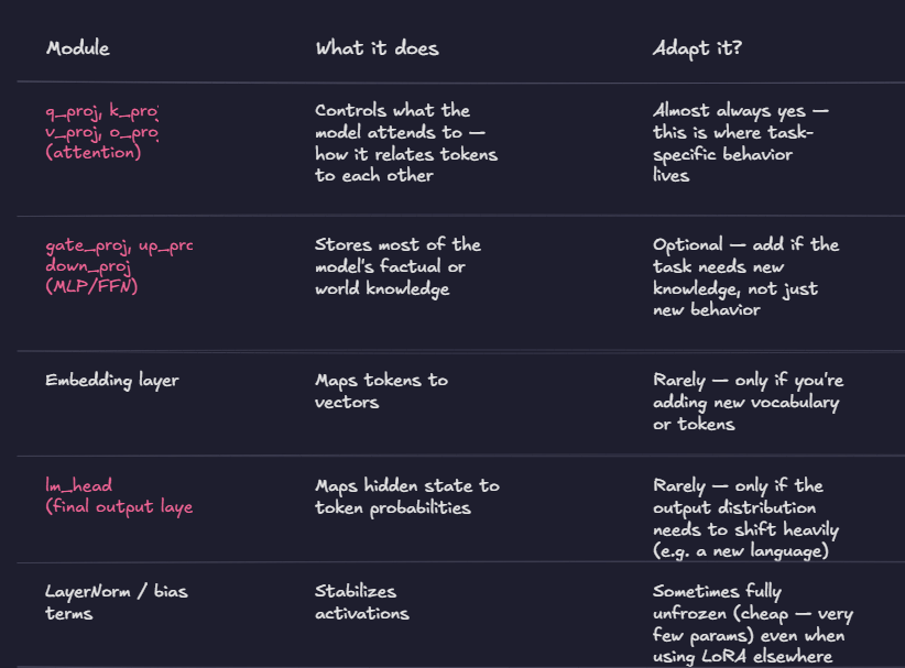
LoRA Adaptation: which modules to target

How do you actually decide?

The reasoning isn’t arbitrary, it comes from what kind of change your task needs:

1. Just changing behavior/style/format (e.g., make it answer in a specific tone, follow a new instruction format) → attention layers only (q,k,v,o). This is the most common setup and matches what you'd use for something like your interview platform's question-generation behavior.
2. Teaching new domain knowledge (e.g., medical terminology, a new coding language) → add the MLP projections too, since that’s where factual associations are stored.
3. Resource-constrained, want max savings → attention-only, smallest footprint, still captures most of the gain (this is the empirical finding from the original LoRA paper — attention-only gets you most of the way there).

Most common practice:

target_modules = ["q_proj", "v_proj"]

(sometimes just Q and V, not all four) and only expand to K, O, and the MLP layers if eval performance shows the model isn’t picking up enough of the task.

Why those ? Because:

• Attention directions change task behavior
• Small adaptation there is very powerful

If dataset is large → apply LoRA to more layers.

If dataset is small → fewer layers.

How Does Quantization Change This? (QLoRA Case)

If you want to understand how Quantization works in depth, you can read this article, https://pub.towardsai.net/understanding-llm-quantization-why-fp32-fp16-bf16-and-int8-matter-for-modern-ai-systems-076ea6eb9ca6

QLoRA’s contribution: quantize the frozen base model down to 4-bit, while keeping the LoRA adapters in higher precision (bf16) for training. This lets you fine-tune a 65B model on a single 48GB GPU instead of needing multiple 80GB A100s.

It’s not a new training method, it’s LoRA + three specific engineering tricks to make the 4-bit quantization not destroy quality or break gradient flow.

The three key innovations

1. NF4 (4-bit NormalFloat) quantization

Standard 4-bit quantization (like FP4 or Int4) assumes values are uniformly distributed. But neural network weights are actually roughly normally distributed (zero-centered, bell curve). NF4 is an information-theoretically optimal data type built specifically for normally-distributed data, it places quantization bins so each bin gets roughly equal probability mass (not equal range), based on quantiles of a N(0,1) distribution.

Practically: weights are first normalized into the range [-1, 1] (by scaling with absolute max), then mapped to one of 16 possible NF4 values that were precomputed to match a standard normal distribution’s quantiles.

This consistently outperforms standard 4-bit float/int quantization for weight distributions you actually see in trained transformers.

2. Double Quantization (DQ)

Quantization isn’t free, you need quantization constants (the scaling factors, e.g., absolute max per block) to dequantize later. If you quantize in small blocks (QLoRA uses block size 64, for accuracy), you get a lot of these constants, and they’re stored in fp32.

For a 65B model, this constant overhead alone is ~127MB — not huge, but not nothing when you’re squeezing every byte.

Double quantization = quantize the quantization constants themselves. The first-level constants (fp32, one per 64-weight block) get quantized again in blocks of 256, this time to 8-bit, using a second quantization constant for that group. This trims that 127MB down to about 27MB. Small in isolation but consistent with the project’s whole philosophy of fanatically reducing every byte of memory.

3. Paged Optimizers

This one isn’t about model weights at all, it’s about avoiding OOM crashes during training caused by memory spikes, specifically from optimizer states (Adam’s momentum + variance buffers) during gradient checkpointing.

QLoRA uses NVIDIA’s unified memory feature to create “paged” optimizer states. When GPU memory is about to overflow during a spike (e.g., long sequence length triggering a big checkpointing recomputation), pages of the optimizer state automatically get evicted to CPU RAM, and brought back to GPU when needed — just like OS-level paging between RAM and disk. This happens transparently without you writing any extra eviction logic.

How it all fits together at training time, the forward/backward pass

This is the part people often get hazy on, so let’s be precise:

1. Storage: base model weights are stored in NF4 (4-bit), with double-quantized constants.
2. Compute dtype: during forward/backward pass, the 4-bit weights for a given layer are dequantized on-the-fly to bf16 right before the matmul. So computation happens in bf16, but storage stays in 4-bit.
3. LoRA adapters (A, B matrices) are kept and trained in bf16 the whole time — they’re never quantized.
4. Gradients only flow into the LoRA adapter parameters. The base model’s 4-bit weights get no gradient updates at all — they’re purely frozen, used only for the forward computation (dequantized transiently, immediately discarded after use — not materialized in full precision in memory).
5. Backward pass: gradients flow through the frozen (dequantized-on-the-fly) base weights mathematically, but only update A and B.

So memory-wise, during training you hold: 4-bit base weights (tiny) + bf16 LoRA adapters (tiny) + optimizer states for adapters only (tiny) + activations. You never need to hold the full-precision base model or its optimizer states. That’s the whole trick.

Now, you must be thinking, what if Quality gets dropped.

No, Quality, does not collapse. Why ?

You might expect 4-bit base weights to wreck downstream performance, but the QLoRA paper showed fine-tuned NF4+DQ models matched full 16-bit LoRA fine-tuning performance closely across benchmarks. The intuition: the base model’s role is just to provide a fixed, frozen feature transformation — small per-step quantization noise in that frozen transform gets absorbed/compensated for by the adapters during training, especially since LoRA is already operating as a low-rank correction on top.

You load model in 4-bit:

BitsAndBytesConfig(load_in_4bit=True)

Lets work with the code now.

Method 1: Hugging Face transformers + peft + trl (SFTTrainer)

!pip install transformers peft trl datasets accelerate bitsandbytes

import torch
from datasets import load_dataset
from transformers import (
    AutoModelForCausalLM,
    AutoTokenizer,
    BitsAndBytesConfig,
)
from peft import LoraConfig, get_peft_model, prepare_model_for_kbit_training
from trl import SFTTrainer, SFTConfig

MODEL_ID = "meta-llama/Llama-2-7b-hf"
OUTPUT_DIR = "./llama7b-lora-hf"

def main() -> None:
    bnb_config = BitsAndBytesConfig(
        load_in_4bit=True,
        bnb_4bit_quant_type="nf4",
        bnb_4bit_compute_dtype=torch.bfloat16,
        bnb_4bit_use_double_quant=True,
    )

    tokenizer = AutoTokenizer.from_pretrained(MODEL_ID)
    tokenizer.pad_token = tokenizer.eos_token

    model = AutoModelForCausalLM.from_pretrained(
        MODEL_ID,
        quantization_config=bnb_config,
        device_map="auto",
    )
    model = prepare_model_for_kbit_training(model)

    lora_config = LoraConfig(
        r=16,
        lora_alpha=32,
        target_modules=["q_proj", "k_proj", "v_proj", "o_proj"],
        lora_dropout=0.05,
        bias="none",
        task_type="CAUSAL_LM",
    )
    model = get_peft_model(model, lora_config)
    model.print_trainable_parameters()

    dataset = load_dataset("tatsu-lab/alpaca", split="train[:5000]")

    def format_example(ex):
        return {
            "text": (
                f"### Instruction:\n{ex['instruction']}\n\n"
                f"### Response:\n{ex['output']}"
            )
        }

    dataset = dataset.map(format_example)

    trainer = SFTTrainer(
        model=model,
        tokenizer=tokenizer,
        train_dataset=dataset,
        args=SFTConfig(
            output_dir=OUTPUT_DIR,
            num_train_epochs=1,
            per_device_train_batch_size=4,
            gradient_accumulation_steps=4,
            learning_rate=2e-4,
            bf16=True,
            logging_steps=10,
            save_strategy="epoch",
            max_seq_length=1024,
            dataset_text_field="text",
            report_to="none",
        ),
    )

    trainer.train()
    trainer.save_model(f"{OUTPUT_DIR}-final")
    tokenizer.save_pretrained(f"{OUTPUT_DIR}-final")
    print(f"Saved LoRA adapter to {OUTPUT_DIR}-final")

if __name__ == "__main__":
    main()

accelerate launch file.py

Method 2: Explicit QLoRA recipe (4-bit base + LoRA on all linear layers)

!pip install transformers peft trl datasets accelerate bitsandbytes

import torch
import bitsandbytes as bnb
from datasets import load_dataset
from transformers import (
    AutoModelForCausalLM,
    AutoTokenizer,
    BitsAndBytesConfig,
    TrainingArguments,
    Trainer,
    DataCollatorForLanguageModeling,
)
from peft import LoraConfig, get_peft_model, prepare_model_for_kbit_training

MODEL_ID = "meta-llama/Llama-2-7b-hf"
OUTPUT_DIR = "./llama7b-qlora"

def find_all_linear_names(model) -> list[str]:
    """Return the names of every 4-bit linear layer to attach LoRA to."""
    lora_module_names = set()
    for name, module in model.named_modules():
        if isinstance(module, bnb.nn.Linear4bit):
            names = name.split(".")
            lora_module_names.add(names[-1])
    lora_module_names.discard("lm_head")
    return list(lora_module_names)

def main() -> None:
    bnb_config = BitsAndBytesConfig(
        load_in_4bit=True,
        bnb_4bit_quant_type="nf4",
        bnb_4bit_compute_dtype=torch.bfloat16,
        bnb_4bit_use_double_quant=True,
    )

    tokenizer = AutoTokenizer.from_pretrained(MODEL_ID)
    tokenizer.pad_token = tokenizer.eos_token

    model = AutoModelForCausalLM.from_pretrained(
        MODEL_ID,
        quantization_config=bnb_config,
        device_map="auto",
    )
    model = prepare_model_for_kbit_training(model, use_gradient_checkpointing=True)

    lora_cfg = LoraConfig(
        r=64,
        lora_alpha=16,
        lora_dropout=0.1,
        bias="none",
        target_modules=find_all_linear_names(model),
        task_type="CAUSAL_LM",
    )
    model = get_peft_model(model, lora_cfg)
    model.print_trainable_parameters()

    dataset = load_dataset("Abirate/english_quotes", split="train")

    def tokenize(batch):
        out = tokenizer(
            batch["quote"],
            truncation=True,
            padding="max_length",
            max_length=512,
        )
        return out

    dataset = dataset.map(tokenize, batched=True, remove_columns=dataset.column_names)

    collator = DataCollatorForLanguageModeling(tokenizer=tokenizer, mlm=False)

    args = TrainingArguments(
        output_dir=OUTPUT_DIR,
        per_device_train_batch_size=2,
        gradient_accumulation_steps=8,
        learning_rate=2e-4,
        num_train_epochs=1,
        bf16=True,
        optim="paged_adamw_8bit",
        logging_steps=10,
        gradient_checkpointing=True,
        save_strategy="epoch",
        report_to="none",
    )

    trainer = Trainer(
        model=model,
        args=args,
        train_dataset=dataset,
        data_collator=collator,
    )

    trainer.train()
    trainer.save_model(f"{OUTPUT_DIR}-final")
    tokenizer.save_pretrained(f"{OUTPUT_DIR}-final")
    print(f"Saved QLoRA adapter to {OUTPUT_DIR}-final")

if __name__ == "__main__":
    main()

3.) Method 3: Unsloth (Triton-kernel optimized, ~2x faster, ~50% less memory)

!pip install "unsloth[cu121] @ git+https://github.com/unslothai/unsloth.git"

import torch
from datasets import load_dataset
from unsloth import FastLanguageModel
from trl import SFTTrainer, SFTConfig

MODEL_NAME = "unsloth/llama-2-7b"
MAX_SEQ_LEN = 2048
OUTPUT_DIR = "./llama7b-unsloth-lora"

def main() -> None:
    model, tokenizer = FastLanguageModel.from_pretrained(
        model_name=MODEL_NAME,
        max_seq_length=MAX_SEQ_LEN,
        dtype=torch.bfloat16,
        load_in_4bit=True,
    )

    model = FastLanguageModel.get_peft_model(
        model,
        r=16,
        target_modules=[
            "q_proj", "k_proj", "v_proj", "o_proj",
            "gate_proj", "up_proj", "down_proj",
        ],
        lora_alpha=16,
        lora_dropout=0,
        bias="none",
        use_gradient_checkpointing="unsloth",
        random_state=3407,
    )

    dataset = load_dataset("yahma/alpaca-cleaned", split="train[:5000]")

    def format_example(ex):
        return {
            "text": (
                f"### Instruction:\n{ex['instruction']}\n\n"
                f"### Response:\n{ex['output']}"
                + tokenizer.eos_token
            )
        }

    dataset = dataset.map(format_example)

    trainer = SFTTrainer(
        model=model,
        tokenizer=tokenizer,
        train_dataset=dataset,
        args=SFTConfig(
            output_dir=OUTPUT_DIR,
            per_device_train_batch_size=2,
            gradient_accumulation_steps=4,
            num_train_epochs=1,
            learning_rate=2e-4,
            bf16=True,
            logging_steps=10,
            save_strategy="epoch",
            max_seq_length=MAX_SEQ_LEN,
            dataset_text_field="text",
            optim="adamw_8bit",
            warmup_steps=5,
            report_to="none",
        ),
    )

    trainer.train()

    model.save_pretrained_merged(
        f"{OUTPUT_DIR}-final",
        tokenizer,
        save_method="lora",
    )
    print(f"Saved Unsloth LoRA adapter to {OUTPUT_DIR}-final")

if __name__ == "__main__":
    main()

I hope this guide helped you understand LoRA/QLoRA from both a theoretical and practical perspective. If you found it useful, consider sharing it with others and leave your thoughts or questions in the comments. Thanks for reading, and happy fine-tuning!

Follow Jiten Bhalavat and subscribe via email to receive upcoming blogs on AI systems, LLM optimization, and practical machine learning engineering straight into your Mailbox.