Visualizing Millions of Points in Seconds: A Deep Dive Into GPU Accelerated t-SNE

How tsne-cuda Turns a Notoriously Slow Dimensionality Reduction Technique Into a Near Instant Tool

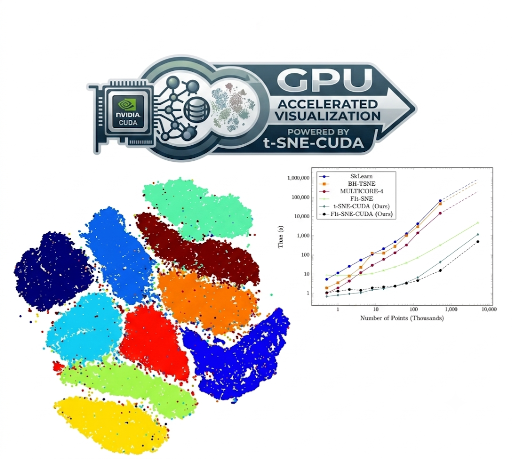
Anyone who has worked with high dimensional data, whether embeddings produced by a neural network, gene expression measurements, or raw pixel data from a large image dataset, has eventually reached for t-SNE. The technique remains one of the most trusted ways to collapse complicated, high dimensional relationships down into a two dimensional scatter plot that a human can actually look at and interpret. Its enduring popularity comes with a well known cost, however: t-SNE is slow, often painfully so, once a dataset grows past a few tens of thousands of points. Waiting fifteen or twenty minutes, or in some cases considerably longer, just to see a visualization of a dataset breaks the natural rhythm of exploratory analysis, where the value often comes from quickly trying several parameter settings or several subsets of data in a row.

tsne-cuda addresses this bottleneck directly by reimplementing the core computation on a GPU. Built as an optimized CUDA based version of the FIt-SNE algorithm, the project reports being able to run up to twelve hundred times faster than the standard scikit learn implementation, and up to fifty times faster than Multicore-TSNE, depending on the dataset and the GPU hardware available. For many practical workflows, the entire migration boils down to a single line of code:

# Before
from sklearn.manifold import TSNE
# After
from tsnecuda import TSNE

Everything downstream of that import, including how the class is constructed and how it is called, follows the same interface already familiar to anyone who has used scikit learn’s implementation, which means adopting the GPU accelerated version rarely requires restructuring an existing analysis pipeline.

Why t-SNE Is Slow in the First Place

To appreciate why a GPU rewrite matters so much here, it helps to understand what makes t-SNE computationally expensive in the first place. The algorithm works by modeling the similarity between every pair of points in the original high dimensional space, then trying to find a low dimensional arrangement of points whose pairwise similarities match as closely as possible. In a naive implementation, this pairwise comparison step scales quadratically with the number of points, meaning that doubling the dataset size roughly quadruples the work involved. Even with clever algorithmic improvements such as the Barnes-Hut approximation, which reduces this to a more manageable but still substantial workload, computing accurate low dimensional embeddings for datasets with hundreds of thousands or millions of points on a standard CPU remains a genuinely heavy computation.

FIt-SNE, the algorithm tsne-cuda builds its CUDA implementation around, introduced further algorithmic improvements using techniques inspired by fast multipole methods and interpolation based approximations, substantially reducing the theoretical cost of the computation. tsne-cuda then takes that already improved algorithm and reimplements its core operations to run on a graphics card rather than a general purpose processor, taking advantage of the sheer number of parallel compute cores a modern GPU offers for exactly the kind of repetitive, parallelizable numerical work that dominates t-SNE’s runtime.

How Much Faster Is It, Really

The project backs its speed claims with benchmark comparisons run against several other widely used implementations, tested across both synthetic datasets and well known public datasets.

On simulated data, generated with fifty dimensions and four underlying clusters, the reported comparisons span a huge range of dataset sizes, from one thousand points up to ten million points, plotted on logarithmic scales for both dataset size and runtime. Because running the slower reference implementations directly at the very largest sizes would take an impractical amount of time, projected timings are used for scikit learn, BH-TSNE, and the four threaded configuration of Multicore-TSNE at the largest scales, based on the expected complexity of an implementation with roughly O(n log n) scaling behavior. Even accounting for that projection at the extreme end, the general shape of the comparison across the full range of tested sizes shows a substantial and growing gap in favor of the GPU implementation as dataset size increases.

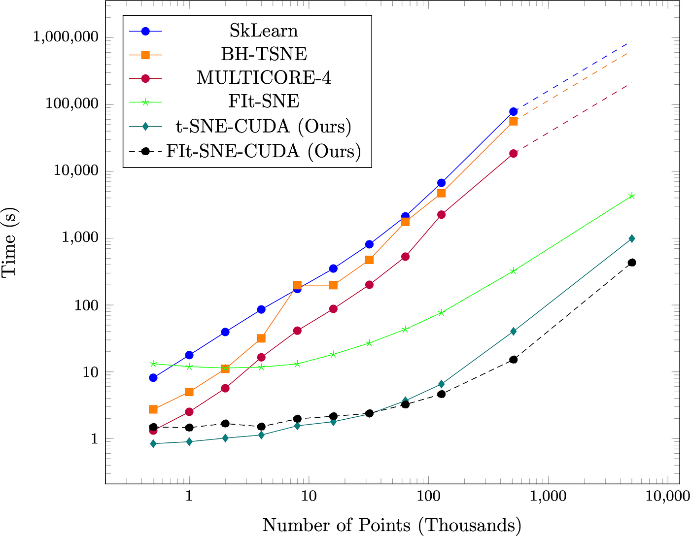
Time taken compared to other state of the art algorithms on synthetic datasets with 50 dimensions and four clusters for varying numbers of points. Note the log scale on both the points and time axis, and that the scale of the x-axis is in thousands of points (thus, the values on the x-axis range from 1K to 10M points. Dashed lines on SkLearn, BH-TSNE, and MULTICORE-4 represent projected times. Projected scaling assumes an O(nlog(n)) implementation.

On the MNIST dataset, a long standing benchmark in the machine learning community consisting of sixty thousand handwritten digit images represented as seven hundred sixty eight dimensional vectors, tsne-cuda completes the full embedding directly on raw pixel values in under seven seconds. For anyone who has previously waited through a scikit learn run on the same dataset, that number alone tends to be the moment the appeal of a GPU implementation becomes obvious.

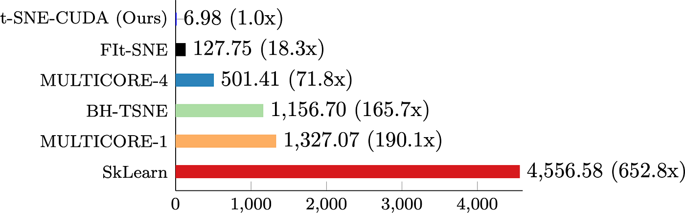
The performance of t-SNE-CUDA compared to other state-of-the-art implementations on the MNIST dataset. t-SNE-CUDA runs on the raw pixels of the MNIST dataset (60000 images x 768 dimensions) in under 7 seconds.

On the CIFAR-10 dataset, using fifty thousand images represented as one thousand and twenty four dimensional feature vectors extracted from a trained classifier rather than raw pixels, tsne-cuda produces an embedding in under six seconds. Running directly on raw CIFAR-10 pixel data instead takes somewhat longer, around twelve seconds, though the resulting embedding tends to be considerably lower quality in that raw pixel case, since Euclidean distance is a relatively poor similarity measure for comparing images directly at the pixel level. This is a useful reminder that speed alone does not solve every part of a t-SNE workflow. Feeding the algorithm a meaningful distance metric, typically by working with learned feature representations rather than raw pixels, still matters a great deal for producing a genuinely useful embedding, regardless of how fast the underlying computation runs.

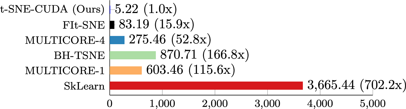
The performance of t-SNE-CUDA compared to other state-of-the-art implementations on the CIFAR-10 dataset. t-SNE-CUDA runs on the output of a classifier on the CIFAR-10 training set (50000 images x 1024 dimensions) in under 6 seconds.

Does Speed Come at the Cost of Quality

A natural and reasonable concern when adopting any accelerated reimplementation of an established algorithm is whether the faster version quietly sacrifices output quality to achieve its speed. The project addresses this directly by comparing the visual output of its GPU implementation against the standard Barnes-Hut implementation and the multithreaded Multicore-TSNE implementation on the MNIST dataset.

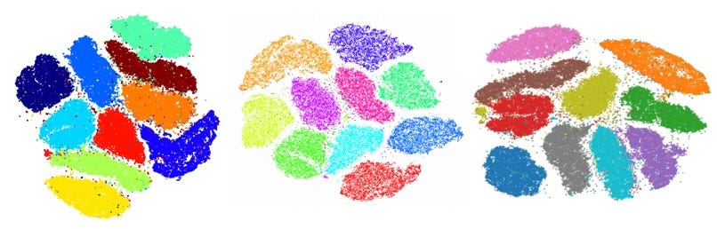
Left: MULTICORE-4 (501s), Middle: BH-TSNE (1156s), Right: t-SNE-CUDA (6.98s).

Side by side comparisons of the resulting cluster structure show visibly comparable groupings and separation between digit classes across all three implementations, despite an enormous difference in runtime: roughly five hundred one seconds for the four threaded Multicore implementation, roughly eleven hundred fifty six seconds for BH-TSNE, and roughly seven seconds for tsne-cuda on the same task. In other words, the reported speed gains do not appear to come from a meaningfully degraded embedding, which is precisely the trade off that would make a faster implementation far less useful in practice regardless of how quickly it ran.

Installing tsne-cuda

Installation options depend somewhat on which CUDA toolkit version is already present on a given machine. For CUDA versions 10.1 and 10.2 specifically, prebuilt binaries are distributed through Anaconda’s conda-forge channel, which is generally the simplest path when it applies:

conda install tsnecuda -c conda-forge

For CUDA version 9.0 and later more broadly, the project supports installation directly from source. Because build requirements and steps can shift somewhat as CUDA toolkits and GPU driver versions evolve, the most current and accurate installation instructions for source based installs are maintained in the project’s wiki rather than duplicated across multiple documents that might drift out of sync with each other. Anyone installing from source should check the wiki directly for the specific combination of CUDA toolkit, compiler, and operating system involved, since GPU library installation is an area where small version mismatches can cause build failures that are otherwise difficult to diagnose.

A general installation guide covering the broader set of supported approaches and dependencies is also maintained directly in the repository, and is the recommended starting point before attempting either the conda based or source based installation path.

Using tsne-cuda in Practice

Once installed, the Python interface deliberately mirrors the widely used scikit learn API for t-SNE, which is a considerable convenience for anyone already familiar with that interface from prior work. Constructing and running the embedding follows essentially the same pattern:

from tsnecuda import TSNE
X_embedded = TSNE(n_components=2, perplexity=15, learning_rate=10).fit_transform(X)

Here, X represents the original high dimensional dataset, typically provided as a two dimensional array where each row is one data point and each column is one feature or dimension. The perplexity parameter controls roughly how many neighboring points are considered when estimating local structure around each point, and is one of the more consequential parameters to tune for a given dataset, since too low a value tends to produce embeddings dominated by noise, while too high a value can blur together genuinely distinct clusters. The learning_rate parameter controls how aggressively the optimization process adjusts the low dimensional coordinates during training, and, like most gradient based optimization settings, benefits from some experimentation on a new dataset rather than blindly reusing a value tuned for a completely different problem.

One notable and deliberate limitation is that n_components currently only supports a value of two, meaning the library only produces two dimensional embeddings rather than three dimensional or higher dimensional ones. The project is explicit that there are currently no plans to support additional output dimensions, since doing so would require substantial changes throughout the underlying implementation rather than a small parameter tweak. For nearly all common visualization use cases, where the entire point of running t-SNE is producing something that can be plotted directly on a two dimensional chart, this limitation tends not to matter in practice, though it is worth knowing in advance for anyone whose workflow specifically depends on a higher dimensional embedding output.

A Typical End to End Workflow

Putting the pieces together, a fairly common analysis pattern looks something like preparing a numeric feature matrix, running the embedding, and then visualizing the result with a plotting library:

import numpy as np
import matplotlib.pyplot as plt
from tsnecuda import TSNE
# Assume X is a NumPy array of shape (n_samples, n_features)
# and labels holds a class label for each sample, used only for coloring the plot
X_embedded = TSNE(
    n_components=2,
    perplexity=30,
    learning_rate=200
).fit_transform(X)
plt.figure(figsize=(8, 8))
plt.scatter(X_embedded[:, 0], X_embedded[:, 1], c=labels, cmap="tab10", s=5)
plt.title("t-SNE Embedding")
plt.show()

Because the underlying computation runs on the GPU rather than the CPU, this same pattern that might otherwise take many minutes on a large dataset can often complete in a matter of seconds, which changes the practical rhythm of exploratory work considerably. Rather than committing to one set of parameters and waiting a long time to see the result, an analyst can reasonably try several perplexity or learning rate values in quick succession and compare the resulting visualizations directly, something that is simply impractical with a slower CPU bound implementation on anything beyond a fairly small dataset.

When GPU Accelerated t-SNE Makes the Most Difference

The size of the speed advantage reported by the project is not uniform across every situation, and it is worth being realistic about when the benefit is most pronounced. On genuinely small datasets, comprising a few thousand points or fewer, even a standard CPU based implementation tends to complete quickly enough that the difference is unlikely to be noticeable in everyday use. The advantage grows substantially as dataset size increases into the tens of thousands, hundreds of thousands, and millions of points, which is precisely the regime where standard implementations become impractically slow or, in the case of extremely large datasets, essentially unusable within a reasonable amount of waiting time. Anyone working primarily with genuinely large embeddings, whether from a large scale genomics dataset, a substantial corpus of learned neural network representations, or a big collection of behavioral or transactional records, stands to benefit the most from adopting a GPU based implementation like this one.

It is also worth noting that meaningful speed gains depend on having access to a reasonably capable GPU and a properly configured CUDA environment. Running exploratory data analysis inside a hosted notebook environment that already provides GPU access, a fairly common setup for many data scientists and researchers today, tends to make adopting this kind of tool almost frictionless, since the underlying hardware and driver setup is typically already handled by the hosting platform.

Choosing Between Raw Features and Learned Representations

The CIFAR-10 comparison mentioned earlier offers a genuinely useful, broader lesson that applies well beyond this particular library. A dimensionality reduction technique, however fast or algorithmically sophisticated, can only produce a meaningful embedding if the distance measure it relies on genuinely reflects meaningful similarity between the original data points. For image data specifically, comparing raw pixel intensities directly using Euclidean distance often fails to capture the kind of semantic similarity a human would recognize immediately, since two images of the same object photographed from slightly different angles or lighting conditions can differ enormously at the pixel level despite being conceptually identical.

Feeding a t-SNE implementation, GPU accelerated or otherwise, with learned feature representations extracted from a trained neural network instead tends to produce embeddings that align far more closely with meaningful, human interpretable categories. This distinction matters regardless of which specific t-SNE implementation a given workflow ultimately uses, and is a useful reminder that raw computational speed and embedding quality are, to a significant degree, separate concerns that both deserve attention.

Practical Tuning Considerations Worth Keeping in Mind

Beyond simply swapping in a faster implementation, getting genuinely useful results from t-SNE, GPU accelerated or otherwise, still depends on a handful of practical habits that tend to separate a helpful visualization from a misleading one. Perplexity is worth treating as a value to sweep across a small range, perhaps trying something like five, fifteen, thirty, and fifty on a new dataset, rather than settling on a single default and assuming the resulting picture is definitive. Different perplexity values can reveal different levels of structure, and comparing a few of them side by side, something that becomes far more feasible once each run only takes a few seconds rather than several minutes, tends to build a more trustworthy overall picture of a dataset’s actual structure.

It is also worth remembering that the distances between clusters in a finished t-SNE plot, and the relative sizes of those clusters, are not reliably meaningful on their own. The algorithm is explicitly designed to preserve local neighborhood relationships rather than global distances, so a large gap between two clusters in the resulting plot does not necessarily indicate a larger real difference than a smaller gap elsewhere. Treating the plot as a tool for spotting which points tend to group together, rather than as a literal, distance preserving map of the original data, tends to avoid a fairly common source of over interpretation.

Finally, since t-SNE’s underlying optimization involves some randomness in its initialization, running the same settings on the same data more than once, particularly when speed is no longer a bottleneck, is a reasonable way to build confidence that an observed clustering pattern is a stable feature of the data rather than an artifact of one particular random starting point. With a GPU accelerated implementation making each individual run inexpensive, this kind of repeated sanity checking becomes a realistic part of a normal workflow rather than an additional cost most analysts would be reluctant to pay.

Conclusion

t-SNE has remained a standard tool for visualizing high dimensional data for years precisely because it tends to produce genuinely interpretable, visually meaningful groupings that simpler linear techniques often miss. Its historical weakness has always been speed, particularly as datasets have grown from thousands of points to millions.

tsne-cuda addresses that weakness directly by reimplementing the core FIt-SNE computation on a GPU, reporting speed improvements as large as twelve hundred times over the standard scikit learn implementation while producing embeddings that remain visually and qualitatively comparable to slower, established alternatives. With an interface intentionally designed to mirror the familiar scikit learn API, adopting the accelerated version in an existing workflow often requires nothing more than changing a single import line.

For anyone regularly working with large scale embeddings, whether from images, genomic data, or learned neural network representations, that kind of speed improvement can genuinely change how exploratory analysis gets done, turning what used to be a long, patience testing wait into something close to an interactive experience.

The repository is available at: https://github.com/CannyLab/tsne-cuda