Global Warming Levels, Explained with Data & Code
A practical CMIP6 and Python walkthrough for moving from years to temperature thresholds.
Global Warming Levels, Explained with Data & Code
A practical CMIP6 and Python walkthrough for moving from years to temperature thresholds.
Photo : Eelco Böhtlingk (@eelco_bohtlingk) / Unsplash
This article presents a reproducible application of the proposed workflow. The cleaned code, preprocessing scripts, and figure-generation routines are available in the accompanying GitHub repository (https://github.com/VSCHY/global_warming_level_illustration).
1. The problem with scenario thinking
Open any IPCC figure and you will see the same alphabet soup: SSP1–2.6, SSP2–4.5, SSP3–7.0, SSP5–8.5. Each “SSP” is a Shared Socioeconomic Pathway, a story about population, technology, and emissions, paired with a radiative-forcing target. Together they span the plausible 21st-century futures climate models simulate.
This diversity is scientifically valuable, but practically complicated. A region might cross +2 °C of warming in 2050 under one scenario and in 2080 under another, yet the physical state of the climate at that warming level (heatwaves, precipitation extremes, sea level rise) is often broadly similar across scenarios. Stakeholders then face a maddening question: which scenario should I plan for?
Global Warming Levels (GWLs) sidestep that question entirely. Instead of asking “what does the climate look like in 2070 under SSP3–7.0?”, they ask “what does the climate look like at +2 °C — whenever and however we get there?”
This shift from a time axis to a temperature axis is the single most useful re-framing of climate projections of the last decade. It is also how IPCC AR6 organises much of its impact science.

Illustration o temperature evolution relative to 1995–2014 and 1850–1900 for different SSP-RCP scenarios up to end of the century. Tebaldi, C., Debeire, K., Eyring, V., Fischer, E., Fyfe, J., Friedlingstein, P., … & Ziehn, T. (2021). Climate model projections from the scenario model intercomparison project (ScenarioMIP) of CMIP6. Earth System Dynamics, 12(1), 253–293.
2. What exactly is a GWL?
A Global Warming Level is just a number of degrees Celsius, typically +1.5 °C, +2 °C, +3 °C, +4 °C, measured as the 20-year mean global surface temperature anomaly relative to the pre-industrial period 1850–1900. Three conventions matter:
- Reference period: 1850–1900. The IPCC and CMIP6 community treat this as the operational pre-industrial baseline. (See preindustrial baseline note at the end, and the IPCC SR1.5 FAQ.)
- Smoothing: 20-year window. A single hot year does not “cross” a GWL. We use a 20-year centred rolling mean to filter out internal variability.
- First-crossing year. For each (model, scenario) pair, the GWL crossing year t is the first year at which the smoothed anomaly reaches the threshold.
Mathematically:


Once you have *t*, you slice the 20-year window centred on t* out of every local field of interest (precipitation, daily maximum temperature, soil moisture …) and treat it as “the local climate at this GWL*”. Pool that across scenarios and you get a multi-scenario distribution of local impacts at, say, +2 °C.
3. Why this is useful
- Stakeholder communication. +2 °C is the language of the Paris Agreement. Decision-makers do not need to learn the difference between SSP2–4.5 and SSP3–7.0 to use a GWL-based map.
- Cross-model aggregation. A 1.5 °C world looks roughly the same in MPI-ESM and IPSL-CM6A even if they reach 1.5 °C in different years. Pooling on the temperature axis is more physically meaningful than pooling on the time axis.
- Policy linkage. GWLs anchor science directly to the 1.5 °C / 2 °C targets of the Paris Agreement and to the “well below 2 °C” language used in national climate adaptation plans.
- Avoiding scenario fatigue. Stakeholders who push back against “you keep changing the scenario” are reassured by a framing that no longer privileges any one socioeconomic story.
4. Method Step-By-Step with an example (Hot days in Toulouse in )
Multiple file have been preprocessed for model CNRM CM6 1 and are available in the following github repo (https://github.com/VSCHY/global_warming_level_illustration), in the data folder.
Inputs are CMIP6 outputs from the Copernicus Climate Data Store (CDS): monthly tas (average surface temperature) for the global mean, daily tasmax (maximum daily temperature) for hot days. These variables were downloaded and preprocessed (conversion into the right unit and calculation of global annual average temperature) for the present exercise
- gmst_annual.csv: global mean surface temperature in °C for different scenarios. Each future scenario is completed with historical time series from the same model. There can be some bias between temperature simulated by the model and historical temperature, see note at the end.
- tasmax_daily.csv: time series of daily maximum temperature over a given location (here Toulouse) in the different scenarios from 1980 to 2100 (each scenario is completed with historical scenario).
4.1 Preprocessing GMST
- We apply the 20 years centred rolling mean,
- We substract the 1850–1900 baseline average,
- We evaluate the first crossing for each GWL (+1.0, 1.5, 2.0, 3.0 °C) on each scenarios, (if GWL is not crossed in a given scenario, then no time windows is considered from it )
- This gives us the 20-yr window relevant for the local impact metric, in each scenarios and for each GWL
import pandas as pd

# Global warming levels to evaluate
GWLS = [1.0, 1.5, 2.0, 3.0]

# Load GMST data
df = pd.read_csv("gmst_annual.csv")

# Ensure clean ordering
df = df.sort_values(["scenario", "year"]).reset_index(drop=True)

# 1. Compute the 1850–1900 baseline average
baseline = df.loc[df["year"].between(1850, 1900), "gmst_C"].mean()

# 2. Apply the 20-year centred rolling mean per scenario
df["gmst_20yr"] = (
    df.groupby("scenario")["gmst_C"]
      .transform(lambda x: x.rolling(window=20, center=True, min_periods=20).mean())
)

# 3. Subtract the 1850–1900 baseline
df["gmst_20yr_anomaly"] = df["gmst_20yr"] - baseline

# 4. Find the first crossing year and the corresponding 20-year window
gwl_intervals = {}

for scenario, group in df.groupby("scenario"):
    gwl_intervals[scenario] = {}

    for gwl in GWLS:
        crossed = group[group["gmst_20yr_anomaly"] >= gwl]

        if crossed.empty:
            # No time window is considered if the GWL is not reached
            gwl_intervals[scenario][gwl] = None
        else:
            first_crossing_year = int(crossed.iloc[0]["year"])

            # With pandas rolling(window=20, center=True),
            # the 20-year window labelled at year Y corresponds to:
            # Y - 9 through Y + 10
            start_year = first_crossing_year - 9
            end_year = first_crossing_year + 10

            gwl_intervals[scenario][gwl] = {
                "crossing_year": first_crossing_year,
                "interval": (start_year, end_year)
            }

gwl_intervals
This allows us to obtain the relevant interval for each GWL for each scenario. Please note that +1°C is only there to display the approximative value for present period.
{
    "ssp1_2_6": {
        1.0: {"crossing_year": 2013, "interval": (2004, 2023)},
        1.5: {"crossing_year": 2028, "interval": (2019, 2038)},
        2.0: {"crossing_year": 2060, "interval": (2051, 2070)},
        3.0: None
    },
    "ssp2_4_5": {
        1.0: {"crossing_year": 2014, "interval": (2005, 2024)},
        1.5: {"crossing_year": 2031, "interval": (2022, 2041)},
        2.0: {"crossing_year": 2049, "interval": (2040, 2059)},
        3.0: {"crossing_year": 2085, "interval": (2076, 2095)}
    },
    "ssp3_7_0": {
        1.0: {"crossing_year": 2014, "interval": (2005, 2024)},
        1.5: {"crossing_year": 2033, "interval": (2024, 2043)},
        2.0: {"crossing_year": 2046, "interval": (2037, 2056)},
        3.0: {"crossing_year": 2067, "interval": (2058, 2077)}
    },
    "ssp5_8_5": {
        1.0: {"crossing_year": 2014, "interval": (2005, 2024)},
        1.5: {"crossing_year": 2029, "interval": (2020, 2039)},
        2.0: {"crossing_year": 2041, "interval": (2032, 2051)},
        3.0: {"crossing_year": 2059, "interval": (2050, 2069)}
    }
}
Annual Mean Global Mean Surface Temperature per scenario in CNRM CM6 1 model (CMIP6).

20 year moving average Mean Global Mean Surface Temperature anomaly compared to 1850–1900 per scenario in CNRM CM6 1 model (CMIP6).

First crossing year for different Global Warming Level across scenario in CNRM CM6 1 model (CMIP6).
4.2 Preprocessing tasmax daily / hot days
Calculate the hot days indicator as the annual number of days with maximum temperature above 35°C.
import pandas as pd

THRESHOLD_C = 35.0

def hot_days_annual(
    tasmax_daily: pd.DataFrame,
    threshold_c: float = THRESHOLD_C
) -> pd.DataFrame:
    """
    Count the number of days per year where daily maximum temperature
    exceeds the threshold.

    Parameters
    ----------
    tasmax_daily : pd.DataFrame
        Daily tasmax data with columns:
        - date
        - scenario
        - tasmax_C

    threshold_c : float
        Temperature threshold in °C.

    Returns
    -------
    pd.DataFrame
        Annual number of hot days per scenario.
    """

    df = tasmax_daily.copy()

    df["date"] = pd.to_datetime(df["date"])
    df["year"] = df["date"].dt.year

    out = (
        (df["tasmax_C"] > threshold_c)
        .groupby([df["scenario"], df["year"]])
        .sum()
        .rename("hot_days")
        .reset_index()[["year", "scenario", "hot_days"]]
        .astype({"hot_days": int})
        .sort_values(["scenario", "year"])
        .reset_index(drop=True)
    )

    return out

tasmax_daily = pd.read_csv("tasmax_daily.csv")

hot_days = hot_days_annual(tasmax_daily, threshold_c=35.0)

hot_days.head()
year scenario hot_days
0 1980 ssp1_2_6 0
1 1981 ssp1_2_6 0
2 1982 ssp1_2_6 0
3 1983 ssp1_2_6 0
4 1984 ssp1_2_6 04.3 Hot days within each GWL window
Once the GWL intervals have been computed from GMST, we use them to select the corresponding 20-year periods in the annual hot-days series.
def hot_days_by_gwl(
    hot_days: pd.DataFrame,
    gwl_intervals: dict
) -> tuple[dict, pd.DataFrame]:
    """
    Aggregate annual hot days over the 20-year GWL windows.

    Parameters
    ----------
    hot_days : pd.DataFrame
        Annual hot-days data with columns:
        - year
        - scenario
        - hot_days

    gwl_intervals : dict
        Nested dictionary containing, for each scenario and GWL,
        the crossing year and associated 20-year interval.

    Returns
    -------
    tuple[dict, pd.DataFrame]
        - Nested dictionary with hot-days statistics by scenario and GWL.
        - Long-format summary dataframe.
    """

    records = []
    hot_days_gwl = {}

    for scenario, gwls in gwl_intervals.items():
        hot_days_gwl[scenario] = {}

        for gwl, info in gwls.items():

            if info is None:
                hot_days_gwl[scenario][gwl] = None
                continue

            start_year, end_year = info["interval"]

            subset = hot_days[
                (hot_days["scenario"] == scenario)
                & (hot_days["year"].between(start_year, end_year))
            ]

            result = {
                "crossing_year": info["crossing_year"],
                "interval": (start_year, end_year),
                "n_years": int(subset["year"].nunique()),
                "mean_hot_days_per_year": float(subset["hot_days"].mean()),
                "median_hot_days_per_year": float(subset["hot_days"].median()),
                "min_hot_days_per_year": int(subset["hot_days"].min()),
                "max_hot_days_per_year": int(subset["hot_days"].max()),
                "total_hot_days_over_window": int(subset["hot_days"].sum()),
            }

            hot_days_gwl[scenario][gwl] = result

            records.append({
                "scenario": scenario,
                "GWL_C": gwl,
                "crossing_year": info["crossing_year"],
                "start_year": start_year,
                "end_year": end_year,
                **result,
            })

    summary = pd.DataFrame(records)

    return hot_days_gwl, summary

hot_days_gwl, hot_days_gwl_summary = hot_days_by_gwl(
    hot_days=hot_days,
    gwl_intervals=gwl_intervals
)

Distribution of Days above 35°C in Toulouse for each GWL acrosse all scenarios with average over the different scenarios, the pooled mean and the median.
5. Limits and outlook
GWLs are powerful but not magic.
- Pattern scaling assumption. Pooling impacts on the temperature axis assumes that, at a given GWL, regional climate signals are similar across scenarios. This is roughly true for slow-responding fields (mean temperature, precipitation climatology) and less true for processes with different transient vs equilibrium responses (e.g. monsoons, ocean circulation, ice-sheet feedbacks).
- Internal variability. With a 20-year window and a handful of scenarios, sampling uncertainty is real. Larger initial-condition ensembles narrow it.
- Model spread is hidden. We pooled across scenarios for one model. A complete GWL analysis runs across multiple CMIP6 models, then reports the multi-model distribution.
Looking ahead, GWLs are now one of the key coordinate in the IPCC AR6 Interactive Atlas, in the European C3S adaptation toolkits, and in impact frameworks such as climada. Expect to see more national adaptation plans expressed in degrees rather than scenarios over the next few years.
References
- Seneviratne, S. I. et al. (2021). Weather and climate extreme events in a changing climate. Climate change 2021: The physical science basis: Working group I contribution to the sixth assessment report of the intergovernmental panel on climate change, 1513–1766. https://www.ipcc.ch/report/ar6/wg1/chapter/chapter-11/
- IPCC SR1.5 (2018), FAQ Chapter 1. Establishes 1850–1900 as the operational pre-industrial baseline. https://www.ipcc.ch/sr15/faq/faq-chapter-1/
- IPCC AR6 WG1 Technical Summary. Confirms 1850–1900 as the reference. https://www.ipcc.ch/report/ar6/wg1/
- Hauser et al.(2022). Transient global warming levels for CMIP5 and CMIP6 (v0.3.0). Zenodo. https://doi.org/10.5281/zenodo.7390473
- Ruane et al. (2024). Non-linear climate change impacts on crop yields may mislead stakeholders. Earth’s Future, 12, e2023EF003842. https://doi.org/10.1029/2023EF003842
Note on preindustrial baseline:
Why anomalies, not absolute temperatures. The whole methodology works on ΔT relative to 1850–1900, never on the raw GMST. That is deliberate: CNRM-CM6–1’s own 1850–1900 mean GMST is about 12.9 °C, roughly 0.9 °C below the observation-based pre-industrial value (~13.7 °C in HadCRUT5). Different CMIP6 models sit on different sides of that observation by ±1 °C or more. Working in anomalies makes those absolute-value biases cancel: a “+2 °C world” in model A is comparable to a “+2 °C world” in model B even when the two disagree about the absolute temperature of either. Applications that do need absolute temperatures (crop-yield emulators, hydrology with non-linear thresholds) need bias correction against an observational baseline before use, the GWL framework deliberately sidesteps that problem rather than solving it.
메타데이터
- post_id
- 0322f9f8fdb3
- slug
- global-warming-levels-explained-with-data-code-0322f9f8fdb3
- url
- https://medium.com/@schrapff.ant/global-warming-levels-explained-with-data-code-0322f9f8fdb3
- canonical_url
- https://medium.com/@schrapff.ant/global-warming-levels-explained-with-data-code-0322f9f8fdb3
- author_url
- https://medium.com/@schrapff.ant
- status
- ok
- fetched_at
- 2026-06-09 15:37:30