The Physics of Async Systems

Understanding the runtime mechanics of event loops, I/O completion, and future orchestration.

Introduction

Async/await presents a linear, almost deceptive model of execution. Code appears to pause and resume seamlessly, as if the runtime simply “waits” and continues. In reality, nothing is waiting. There is no paused thread holding your stack. What exists instead is a coordinated system of state machines, queues, schedulers, and kernel interfaces that collectively simulate this behavior.

Every await splits your function into segments. The compiler lifts its state into a heap-allocated frame, converts control flow into an explicit state machine, and hands execution over to an executor. Progress is no longer implicit—it depends on external signals: I/O readiness, timer expiry, or explicit wakeups. These signals propagate through wakers into run queues, are scheduled by executors, and eventually drive the coroutine forward through repeated polling.

This article builds a complete mental model of that system. It connects the layers that are usually explained in isolation — event loops, I/O backends, promises, coroutines, schedulers — into a single execution pipeline. The focus is not on how to use async, but on how it actually works: the data structures, invariants, and ordering guarantees that determine correctness and performance.

Topics

Async runtimes = tightly coupled subsystems

Designed to optimize latency, throughput, memory efficiency, and correctness under concurrency.

Event Loop (core orchestrator)

• Manages execution using ring buffers (ready queue)
• Uses heaps or timing wheels for timers
• Defines execution order via phases and microtask draining

I/O Layer (kernel interaction)

• Uses models like epoll or io_uring
• Converts blocking operations → completion events
• Optimizes via shared-memory rings and batched syscalls

Promise / Future System

• Shared state with atomic transitions
• Stores continuations for chaining
• Guarantees single resolution + controlled scheduling

Stackless Coroutines (compiler transformation)

• async/await → state machine
• Heap-allocated frame stores execution state
• Progress driven via poll() and suspension points

Scheduler / Executor (execution engine)

• Work-stealing deques + global queues
• Optimizes locality and load balancing
• Uses cooperative scheduling (task budgeting)

Wakers (rescheduling mechanism)

• Decoupled notification system
• Allows tasks to be resumed without executor awareness
• Requires strict ordering to avoid lost wakeups

Channels (task communication)

• Lock-free, sequence-based queues
• High-throughput message passing
• Integrated with async park/wake logic

Backpressure (flow control)

• Token bucket, GCRA, adaptive concurrency
• Regulates load based on rate or latency
• Prevents overload without blocking

Cancellation (termination semantics)

• Two-phase protocol (signal + cleanup)
• Requires safe interruption guarantees
• Distinguishes safe vs unsafe cancellation points

Overall Model A non-blocking, event-driven system where:

• progress is explicit
• state is externalized
• correctness depends on precise coordination across subsystems

1. Event Loop Internals

The event loop is the beating heart of every async runtime. Understanding its internal data structures is not optional — every performance characteristic, every ordering guarantee, every subtle bug you will ever encounter in async code traces back to how the event loop is built.

Ring Buffer — The Ready Event Queue

The event loop needs a queue to hold tasks that are ready to run. The naive choice is a dynamic array or linked list. Both are wrong for this use case.

A dynamic array reallocates on growth — you cannot predict when, and the reallocation causes an O(n) copy at the worst possible moment. A separately-allocated linked list requires a heap allocation per node — under high event throughput this means thousands of allocations per second, destroying cache locality and creating GC pressure.

The ring buffer solves both. It is a fixed-size circular array with two indices — head and tail. Push advances tail, pop advances head. Both wrap around using modulo (or bitmask if the size is a power of two, which is always preferred because bitmask is a single AND instruction versus a division).

push(item):
    data[tail % N] = item
    tail++

pop():
    if head == tail: return EMPTY
    item = data[head % N]
    head++
    return item

The critical property: zero allocation after initialization. The buffer is allocated once. Every push and pop is O(1) with no heap involvement. The entire buffer fits in cache after warmup. This matters because the event loop runs this queue thousands of times per second — any per-operation allocation cost compounds catastrophically.

Participant A      Participant B      Participant C
     |                   |                   |
     |---- Request ----->|                   |
     |                   |---- Process ----->|
     |                   |<--- Response -----|
     |<--- Reply --------|                   |
     |                   |                   |

The second critical property: predictable memory usage. A dynamic queue can grow without bound if producers outrun consumers. A ring buffer enforces a hard capacity — if the ready queue is full, you have a backpressure problem that must be surfaced, not silently absorbed by allocating more memory.

Min-Heap — The Timer Queue

The event loop must fire timers at the correct time. The data structure holding pending timers must answer one question efficiently: what is the next timer to expire?

A min-heap answers this in O(1) — the minimum is always at index 0. Insertion and removal are O(log n). For typical timer counts (hundreds to low thousands), log n is effectively constant.

struct Timer:
    expiry_time
    callback

sift_up(i):
    while i > 0:
        parent = (i - 1) / 2
        if data[parent].expiry > data[i].expiry:
            swap(data[parent], data[i])
            i = parent
        else: break

sift_down(i):
    loop:
        left    = 2*i + 1
        right   = 2*i + 2
        smallest = i
        if left  < len and data[left].expiry  < data[smallest].expiry: smallest = left
        if right < len and data[right].expiry < data[smallest].expiry: smallest = right
        if smallest == i: break
        swap(data[i], data[smallest])
        i = smallest

Why a heap and not a sorted array? Insertion into a sorted array is O(n) — you must shift elements. Under high timer churn (network timeouts being set and cancelled constantly), O(n) insertion kills throughput. The heap gives O(log n) for both insert and delete.

Why not a balanced BST (red-black tree)? A BST gives the same asymptotic complexity but has worse constants — each node is separately allocated, pointer-chasing kills cache locality. The heap is a contiguous array — sift operations walk a predictable path through contiguous memory.

The event loop uses the heap’s minimum to set the epoll_wait timeout. This is the integration point between the timer system and the I/O notification system:

timeout = timer_heap.peek().expiry - now
events  = epoll_wait(timeout)

If no I/O events arrive, epoll_wait returns after exactly timeout nanoseconds — and the loop fires the expired timer. This means the loop never busy-waits and never sleeps longer than the next timer requires. Getting this right is what makes a runtime both CPU-efficient and timer-accurate simultaneously.

Hierarchical Timing Wheel — High-Scale Timers

The min-heap breaks down at scale. With tens of thousands of concurrent timers (one per TCP connection timeout, one per request deadline, one per keepalive), O(log n) insert becomes measurable. More critically, timer cancellation in a heap requires finding the node first — O(n) scan unless you maintain a separate index.

The hierarchical timing wheel solves this. It trades the heap’s generality for O(1) insert, O(1) cancel, and O(1) amortized expire — at the cost of quantized resolution.

The structure: multiple arrays (wheels), each representing a different time granularity. Level 0 has slots of 1ms each, 256 slots covering 256ms. Level 1 has slots of 256ms each, covering 65 seconds. Level 2 covers hours. Each slot holds a linked list of timers expiring in that slot’s window.

insert(timer, delay):
    for level in levels:
        if delay < level.tick_duration * SLOTS:
            slot = (level.cursor + delay / level.tick_duration) % SLOTS
            level.buckets[slot].append(timer)
            return
        delay -= remaining time at this level

tick():
    levels[0].cursor++
    fire all timers in levels[0].buckets[cursor]
    if levels[0].cursor wrapped:
        cascade from levels[1] into levels[0]
        levels[1].cursor++
        if levels[1].cursor wrapped:
            cascade from levels[2] ...

The cascade is the key operation. When level 0’s cursor wraps around (every 256ms), it pulls all timers from the current slot of level 1, re-inserts them into level 0 at their precise sub-slot. This amortizes the work across all 256 ticks of level 0 — a single cascade is O(k) where k is the number of timers in that level-1 slot, but averaged across 256 ticks it approaches O(1).

Cancellation is O(1): each timer node is in a linked list. If you hold a pointer to the node (which the setTimeout return value gives you), removal is pointer manipulation — no searching required.

This is why Linux’s kernel timer implementation, Netty’s HashedWheelTimer, Kafka's Timer, and Tokio's timer all use wheels rather than heaps. The constant factors matter at the scale these systems operate at.

Intrusive Linked List — The Run Queue

The ready-to-run queue inside the event loop has a constraint the ring buffer does not satisfy: tasks must be able to remove themselves from the middle of the queue (for cancellation), and the queue must handle arbitrary growth without reallocation.

The intrusive linked list solves this by embedding the list node directly inside the task struct:

struct Task:
    next: *Task          // the list pointer lives inside the task
    prev: *Task
    callback
    state

Non-intrusive lists allocate a separate list node that holds a pointer to the element. This means two heap allocations per enqueue: one for the node, one for the element. The intrusive version allocates the task once — the list node is part of the task’s memory. Enqueue and dequeue are pure pointer manipulation, zero allocation.

The second advantage: given a pointer to a task, you can remove it from any list in O(1) without knowing which list it is in — just manipulate its own prev/next pointers. This is essential for cancellation: when a timeout fires and cancels a pending I/O operation, the operation’s task must be removed from whatever queue it currently occupies, immediately, without searching.

This is why the Linux kernel uses intrusive lists (list_head embedded in every kernel data structure) for virtually everything. The pattern appears in every high-performance runtime for the same reasons.

Phase Ordering and Microtask Draining

The event loop is not a simple while loop. It has phases, and the ordering of those phases determines the observable execution order of all async code. Getting this wrong produces bugs that are nearly impossible to reason about from the outside.

The canonical phase structure:

loop:
    phase: timers         — fire all expired setTimeout / setInterval
    drain microtask queue
    phase: pending I/O    — fire I/O callbacks deferred from previous iteration
    drain microtask queue
    phase: poll           — block on epoll_wait, fire ready I/O callbacks
    drain microtask queue
    phase: check          — fire setImmediate callbacks
    drain microtask queue
    phase: close          — fire close event callbacks
    drain microtask queue

The microtask drain between every phase is the critical invariant. Microtasks (Promise continuations, queueMicrotask) must run to completion before the event loop advances to the next phase. This is why promise chains always complete before the next timer fires, even a timer with delay 0.

drain_microtask_queue():
    while not microtask_queue.empty():
        fn = microtask_queue.pop_front()
        fn()  // fn may enqueue more microtasks — keep draining

Note that draining is recursive in the sense that each callback may enqueue more microtasks, which are also drained before returning. This means an infinite microtask chain will starve the I/O phase entirely — the loop never advances. This is not a theoretical concern: it is the mechanism behind one of the most common async performance bugs.

The phase ordering also explains why setImmediate (check phase) fires before a setTimeout(fn, 0) (timers phase) when both are queued from within an I/O callback (poll phase) — after poll, check comes before the next timers phase.

2. I/O Submission and Completion — io_uring

io_uring represents a fundamental rethinking of how userspace and the kernel communicate about I/O. The traditional model (epoll + read/write) requires at minimum two syscalls per I/O operation: one to learn the fd is ready, one to perform the actual transfer. Each syscall is a privilege level transition — roughly 100–1000ns of overhead on modern CPUs with Spectre/Meltdown mitigations. At 100k operations per second, syscall overhead alone consumes 10–100ms of CPU time per second.

io_uring eliminates this entirely for the steady-state fast path.

The Ring Pair — Shared Memory Between Userspace and Kernel

The architecture is two lock-free ring buffers in shared memory — mapped into both userspace and kernel address space via mmap. No data is copied between them. Both sides read and write to the same physical memory pages.

struct SubmissionQueue:
    entries: SQE[]          // array of submission queue entries
    head:    atomic_u32     // kernel reads from head — consumer
    tail:    atomic_u32     // userspace writes to tail — producer
    mask:    u32            // capacity - 1, for fast modulo

struct CompletionQueue:
    entries: CQE[]
    head:    atomic_u32     // userspace reads from head — consumer
    tail:    atomic_u32     // kernel writes to tail — producer
    mask:    u32

Userspace submits work by writing SQEs (submission queue entries) into the SQ array at the current tail position, then advancing the tail with a release store. The kernel sees the new tail via its own view of the same memory and processes the entries.

The kernel writes CQEs (completion queue entries) into the CQ array and advances the CQ tail. Userspace polls the CQ head to harvest completions.

The release/acquire memory ordering is critical. The producer’s store of data must be visible to the consumer before the store of the tail index — otherwise the consumer reads the index, sees new work, but reads stale data. A release store on the tail, paired with an acquire load on the consumer side, provides exactly this guarantee without a full memory fence.

SQE and CQE — The Communication Protocol

Every I/O operation is described by a 64-byte SQE:

struct SQE:
    opcode:      u8     // READ, WRITE, ACCEPT, CONNECT, SEND, RECV, FSYNC ...
    flags:       u8     // IOSQE_IO_LINK, IOSQE_BUFFER_SELECT, IOSQE_FIXED_FILE ...
    fd:          i32    // file descriptor (or registered file index)
    offset:      u64    // file offset for read/write; 0 for sockets
    buffer_ptr:  u64    // userspace buffer address
    buffer_len:  u32    // buffer length
    user_data:   u64    // opaque — echoed back in CQE; use to correlate completion to submission

The user_data field is the correlation mechanism. When a CQE arrives, you look up the pending operation by user_data to know what completed and with what result. In practice this is an index into a slab of in-flight operation structs.

struct CQE:
    user_data:  u64    // matches SQE.user_data exactly
    result:     i32    // bytes transferred, or negative errno on error
    flags:      u32    // IORING_CQE_F_BUFFER (buffer index in high bits), IORING_CQE_F_MORE

The 64-byte SQE size is deliberate — it fits exactly in one cache line. Writing an SQE is a single cache line write with no false sharing against adjacent SQEs.

Batched Submission — Eliminating Syscall Per Operation

The naive use of io_uring still calls io_uring_enter once per operation. The correct use accumulates all SQEs for a tick of the event loop, then submits them all with a single io_uring_enter:

pending = []

enqueue_read(fd, buf, len, token):
    pending.append(SQE(opcode=READ, fd=fd, buffer_ptr=buf, buffer_len=len, user_data=token))

flush_submissions():
    for sqe in pending:
        sq.entries[sq.tail & sq.mask] = sqe
        sq.tail.store(sq.tail + 1, release)
    io_uring_enter(fd, submit=len(pending), min_complete=0, flags=0)
    pending.clear()

One syscall for N operations. At 32 operations per flush, you reduce syscall overhead by 32x. This is the primary source of io_uring’s throughput advantage over epoll.

Linked SQE Chains — Sequential Async Pipelines in Kernel Space

Setting IOSQE_IO_LINK on an SQE creates a dependency: the next SQE in the submission only executes if the current one succeeds. This allows you to express multi-step I/O sequences as a chain submitted in one batch:

submit_chain([
    SQE(RECV,  fd, buf1, flags=IOSQE_IO_LINK),    // receive request header
    SQE(READ,  file_fd, buf2, flags=IOSQE_IO_LINK), // read file from disk
    SQE(SEND,  fd, buf2, flags=0)                  // send file contents
])

The kernel executes these sequentially without returning to userspace between steps. No wakeup, no scheduling, no syscall between the receive and the send. For the common pattern of “receive request, read data, send response” this eliminates two userspace round-trips per request.

If any SQE in the chain fails, the kernel marks subsequent SQEs with ECANCELED in their CQEs — you still get a CQE for each, you just handle the error path.

Provided Buffers — Eliminating TOCTOU in Buffer Management

The traditional model has a time-of-check to time-of-use (TOCTOU) problem: you learn a fd is readable (check), then you call read with a buffer you must have ready (use). You must pre-allocate buffers before knowing how many fds will become readable simultaneously — either over-allocating or risking buffer unavailability.

Provided buffers invert this. You register a pool of buffers with the kernel upfront. When submitting a RECV, you specify the buffer group ID but no specific buffer. The kernel selects a free buffer from the pool at the moment data arrives, places the data there, and reports which buffer ID was used in the CQE flags.

register_buffers(pool_id, bufs[N]):
    io_uring_register(IORING_REGISTER_PBUF_RING, pool_id, bufs, N)

submit_recv(fd, pool_id, token):
    SQE(opcode=RECV, fd=fd, buf_group=pool_id, flags=IOSQE_BUFFER_SELECT, user_data=token)

on_cqe(cqe):
    buf_id  = cqe.flags >> IORING_CQE_BUFFER_SHIFT
    buf     = pool.get(buf_id)
    process(buf[0 .. cqe.result])
    pool.return(buf_id)

The kernel only consumes a buffer when data actually arrives — never wastes a buffer on a connection with no data. For 10,000 concurrent connections, you need buffers proportional to active connections, not total connections.

3. Promise and Future Machinery

Promises are often described as “a value that will be available in the future.” This description is true but useless for understanding what actually happens. The correct mental model: a promise is a state machine with a linked list of continuations, shared between two handles via a reference-counted heap allocation.

The Shared State — What a Promise Actually Is

Every promise/future pair shares a single heap-allocated struct:

struct SharedState<T, E>:
    state:         atomic enum { PENDING, FULFILLED, REJECTED }
    value:         Option<T>
    error:         Option<E>
    refcount:      atomic_u32
    continuations: IntrusiveList<Continuation>
    mutex:         Mutex                  // guards continuations list

The Promise handle and the Future handle are both thin wrappers around a pointer to this struct. The refcount starts at 2 — one for each handle. When either handle is dropped, the refcount decrements. When it reaches 0, the shared state is freed.

This is why you can pass a future to another thread and resolve the promise from yet another thread — they share the same heap allocation, and the atomic state field ensures only one resolution wins.

One-Shot Resolution — The CAS Guarantee

The most critical property of a promise is that it can only be resolved once. Multiple resolves must be silently dropped — not panicked, not queued, silently dropped. This enables patterns like “resolve from whichever I/O callback fires first” without coordination.

resolve(value):
    expected = PENDING
    if not state.compare_exchange(expected, FULFILLED, acq_rel, acquire):
        return                                    // already settled — drop
    state.value = Some(value)
    flush_continuations()

reject(error):
    expected = PENDING
    if not state.compare_exchange(expected, REJECTED, acq_rel, acquire):
        return
    state.error = Some(error)
    flush_continuations()

The compare-exchange atomically checks that state is still PENDING and transitions to FULFILLED in one uninterruptible operation. The second resolver to call this finds state is no longer PENDING — the CAS fails, and it returns immediately.

The acq_rel ordering on success ensures that the value write before the CAS is visible to any thread that observes the new state via an acquire load. Without this, a consumer could observe FULFILLED but read a stale (uninitialized) value.

Continuation Chain — How .then() Is Stored

When you call .then(on_fulfill, on_reject) on a future, you are not executing anything. You are attaching a continuation to the shared state's continuation list. The continuation will be executed later, when the promise is resolved.

then(on_fulfill, on_reject):
    next_promise, next_future = create_pair()

    cont = Continuation(fn():
        if state.state == FULFILLED:
            result = on_fulfill(state.value)
            assimilate(next_promise, result)
        else:
            result = on_reject(state.error)
            assimilate(next_promise, result)
    )

    lock(state.mutex)
    if state.state == PENDING:
        state.continuations.push(cont)
        unlock(state.mutex)
    else:
        unlock(state.mutex)
        microtask_queue.push(cont)         // already settled — schedule immediately

    return next_future

Two paths: if the promise is still pending, the continuation is stored in the list — it will be enqueued when the promise resolves. If the promise is already settled (another thread resolved it between creation and this .then() call), the continuation is immediately scheduled as a microtask.

The mutex around the continuations list guards against a race: the promise resolves on thread A while .then() is attaching a continuation on thread B. Without the mutex, the resolution flush could walk the list and miss the continuation that is mid-insertion. The continuation would then never run — a silent bug.

Flush — Resolution to Microtask Queue

When a promise resolves, it walks the continuation list and enqueues each continuation as a microtask:

flush_continuations():
    lock(state.mutex)
    list = take(state.continuations)       // atomically steal the entire list
    unlock(state.mutex)
    for cont in list:
        microtask_queue.push(cont)         // schedule, do not execute yet

Critical: flush does not execute continuations directly. It enqueues them as microtasks. Execution happens in the microtask drain phase of the event loop. This ensures two properties:

First, promise callbacks are always asynchronous — .then() never calls your callback synchronously even if the promise is already resolved. This eliminates Zalgo — the pathological behavior where a callback fires synchronously sometimes and asynchronously other times depending on internal state.

Second, the resolution code (which may be deep inside a library) does not directly execute user code. It only enqueues. This prevents re-entrancy: user code cannot call back into the resolver while the resolver is still on the stack.

Thenable Assimilation — Flattening Promise Chains

If .then() returns a value, the next promise is resolved with that value. But if .then() returns another promise, you do not want a promise-of-a-promise — you want the outer promise to wait for the inner one. Thenable assimilation handles this:

assimilate(promise, value):
    if value is PromiseLike:              // has a .then method
        value.then(
            fn(v): promise.resolve(v),
            fn(e): promise.reject(e)
        )
    else:
        promise.resolve(value)

This is recursive in the sense that if value.then also returns a promise, assimilation runs again. The chain flattens to arbitrary depth. Without this, fetch().then(r => r.json()) would return a Promise<Promise<JSON>> instead of a Promise<JSON> — every async operation returning a promise would require explicit unwrapping.

This is why the Promises/A+ specification dedicates more text to the resolution procedure than to any other aspect — thenable assimilation is subtle and the source of many interoperability bugs between promise implementations.

Unhandled Rejection Tracking

A rejected promise with no .catch() is a silent failure. The runtime must detect this and surface it. The mechanism:

reject(error):
    ...settle...
    if state.continuations.empty():
        unhandled_set.add(state)          // no handlers yet — potentially unhandled

then(on_fulfill, on_reject):
    unhandled_set.remove(state)          // handler attached — no longer unhandled
    ...

end_of_microtask_checkpoint():
    for state in unhandled_set:
        emit('unhandledRejection', state.error)
    unhandled_set.clear()

The check happens at the end of the microtask checkpoint — not immediately on rejection. This is essential: it allows code like promise.reject(err); promise.catch(handler) to attach the handler synchronously after rejection without triggering a false unhandled rejection warning. The checkpoint boundary is the point at which the runtime can be certain no more synchronous handler attachment is possible.

The unhandled_set is a weak set — it holds references that do not prevent garbage collection. If the promise itself is collected (nobody holds a reference) before the checkpoint, it is removed from the set automatically. This prevents false positives for promises that are created, rejected, and immediately discarded with no possible handler.

4. Stackless Coroutine State Machine

The stackless coroutine is the single most important transformation in modern async programming. Every async/await in every language compiles down to this. Understanding the transformation at the machine level is what separates engineers who debug async correctly from engineers who guess.

The Core Problem Stackless Coroutines Solve

A regular function has one entry point and one exit point. Its local variables live on the call stack — when the function returns, the stack frame is destroyed. This model is incompatible with suspension: if you suspend in the middle of a function and return control to the caller, the stack frame is gone. When you try to resume, all local variables have been overwritten by subsequent calls.

The stackless coroutine solves this by moving all state that must survive a suspension point off the stack and into a heap-allocated struct — the coroutine frame. The function itself is transformed into a state machine that can be entered at any previously suspended point.

The Compiler Transformation

Consider this async function:

async fn fetch_and_process(url, timeout):
    conn   = await connect(url)
    data   = await read(conn, timeout)
    result = process(data)
    return result

There are two suspension points: await connect and await read. The compiler identifies every local variable that is alive across any suspension point. Here conn is alive across await read (it is used after the first await). data is alive across nothing (process runs before any suspension after the second await, but process itself is synchronous). url and timeout are parameters — alive from the start.

The compiler generates:

struct FetchAndProcessFrame:
    state:   enum { START, AFTER_CONNECT, AFTER_READ, DONE }
    url:     String          // alive from start — must survive first suspension
    timeout: Duration
    conn:    Connection      // alive across second suspension — must be stored
    connect_future: ConnectFuture     // the sub-future being awaited at state 0
    read_future:    ReadFuture        // the sub-future being awaited at state 1

Note: data and result do not appear in the frame — they are only live within a single phase and can be stack-allocated within that phase's execution.

The poll function:

poll(frame, waker):
    switch frame.state:

        case START:
            frame.connect_future = connect(frame.url)
            frame.state = AFTER_CONNECT
            // fall through to poll the sub-future immediately

        case AFTER_CONNECT:
            match frame.connect_future.poll(waker):
                Ready(conn):
                    frame.conn = conn
                    frame.read_future = read(frame.conn, frame.timeout)
                    frame.state = AFTER_READ
                    // fall through to poll read_future immediately
                Pending:
                    return Pending

        case AFTER_READ:
            match frame.read_future.poll(waker):
                Ready(data):
                    result = process(data)
                    frame.state = DONE
                    return Ready(result)
                Pending:
                    return Pending

        case DONE:
            panic("polled after completion")

This is the complete transformation. The switch-on-state is the resume mechanism. Each case resumes at the exact point the coroutine last suspended. The fall-through from START to AFTER_CONNECT to AFTER_READ handles the case where sub-futures complete synchronously — no unnecessary yield to the executor.

Frame Layout and Memory

The frame struct is heap-allocated when the coroutine is spawned as a task. Its size is computed at compile time — the compiler knows exactly which variables are alive at each suspension point and packs them into the struct.

A critical optimization: variables that are never alive simultaneously across a suspension point can share the same memory location. This is a union-like optimization — the frame uses max(size_of_branch_A, size_of_branch_B) bytes for variables that are mutually exclusive.

// if conn is only used between suspension 1 and 2,
// and result is only used after suspension 2,
// they can overlap in the frame:

union:
    conn:   Connection      // alive between state 1 and 2
    result: ProcessResult   // alive after state 2 (before return)

This makes coroutine frames significantly smaller than naive analysis suggests. In Rust, the compiler performs this optimization automatically — the future size is the minimum necessary to represent all live variable sets simultaneously.

The frame also contains the nested future slots (connect_future, read_future). These are stored inline in the parent frame — not separately heap-allocated. This means a chain of 10 awaits produces one heap allocation for the outermost frame, which contains all nested frames inline. The entire async call chain is a single contiguous allocation.

The Waker — Scheduling Without an Executor Reference

When a sub-future cannot complete immediately, it must somehow notify the executor to re-poll the parent future when it can make progress. The sub-future cannot hold a direct reference to the executor — that would create a circular dependency and require knowing which executor is being used at future construction time.

The Waker abstracts this:

struct Waker:
    data:   *void              // opaque pointer — executor-defined
    vtable: *WakerVTable

struct WakerVTable:
    wake:         fn(*void)    // consume the waker and schedule the task
    wake_by_ref:  fn(*void)    // schedule the task without consuming
    clone:        fn(*void) -> Waker
    drop:         fn(*void)

The executor creates a Waker for each task before polling it. The Waker’s data pointer points to the task struct. The wake function, when called, pushes the task back onto the executor's run queue.

The sub-future stores this waker when it returns Pending:

// inside ConnectFuture.poll:
poll(frame, cx):
    if socket_ready:
        return Ready(conn)
    else:
        io_source.register_waker(cx.waker.clone())  // store waker in the I/O interest table
        return Pending

When the socket becomes readable, the I/O driver retrieves the stored waker and calls wake(). This enqueues the parent task without the sub-future needing to know anything about which executor is running or how scheduling works.

The vtable indirection is what makes this work across executor implementations. The same future code runs identically whether the executor is single-threaded, multi-threaded, or a custom embedded runtime — the waker’s vtable contains all executor-specific behavior.

Waker Registration — The Critical Ordering

The order of operations inside a future’s poll is not arbitrary. The correct order is:

poll(frame, cx):
    result = attempt_operation()        // 1. try the operation first
    if result == WOULD_BLOCK:
        register_waker(cx.waker)        // 2. only register if it would block
        result = attempt_operation()    // 3. try again after registering
        if result == WOULD_BLOCK:
            return Pending              // 4. now safe to return Pending
    return Ready(result)

Why the second attempt after registration (step 3)? Because the event that would have triggered the waker may have occurred between step 1 and step 2. If you register and then check, you close this window — if the event happened between steps 1 and 2, step 3 will succeed. If you only check before registering, you return Pending with a waker that will never be called because the event already fired.

This is one of the most subtle correctness requirements in async runtime implementation. A future that gets this wrong produces a task that suspends permanently — it returned Pending, the waker was never called, the task is never re-polled, the operation never completes. From the outside it looks like a hang with no error.

HALO — Heap Allocation Elision

The heap allocation for coroutine frames is the main cost of async in languages like Rust. HALO (Heap Allocation Elision Optimization) eliminates this cost when the compiler can prove the future is immediately awaited without being moved or stored.

The conditions for elision:

• The future is created and awaited in the same expression: await connect(url)
• The future is never stored in a struct or passed to a function that might store it
• The future’s size is known at compile time (always true for stackless)

When these hold, the compiler allocates the nested future’s frame directly within the parent frame, on the parent’s stack or within the parent’s heap allocation. Zero additional heap operations.

// This:
let conn = await connect(url)

// Compiles to frame inline storage, no heap alloc for connect's frame:
frame.connect_future = connect(url)   // stored inside parent frame directly
poll(frame.connect_future, cx)

In practice, well-written async code achieves near-zero allocation per await point after the initial task spawn. The entire async call tree is one allocation.

The Colored Functions Problem — Why It Matters

Stackless coroutines have a fundamental limitation: suspension can only happen at explicit await points, and await can only appear inside an async function. A synchronous function cannot contain an await. This means if any function in your call chain needs to await something, every function above it must also be async.

async fn a(): await b()
async fn b(): await c()
async fn c(): await some_io()

// sync_fn cannot call a() and wait for it without blocking a thread:
fn sync_fn():
    result = block_on(a())   // forces blocking — defeats async

This “coloring” of functions — async vs sync — propagates upward through the entire call stack. It means you cannot add async I/O to a deeply nested function without making the entire call chain async. It is a viral property.

This is not a solvable problem within the stackless model — it is an inherent consequence of the design. Stackful coroutines (goroutines, virtual threads) avoid this entirely because they carry a real stack and can suspend from any call depth. The tradeoff is that stackful coroutines are heavier — each requires its own stack allocation regardless of whether it ever suspends.

The existence of this problem is why Go chose stackful goroutines, why Java Loom chose virtual threads with real stacks, and why some Rust users reach for tokio::task::spawn_blocking when integrating with sync libraries — to run sync code on a thread pool where it can block without harming the async executor.

5. Scheduler and Executor Internals

The executor is the runtime that drives futures to completion. Its internal design determines throughput, latency, fairness, and CPU utilization. The data structures and algorithms here are directly responsible for the performance characteristics you observe in production.

Work-Stealing Deque — The Chase-Lev Algorithm

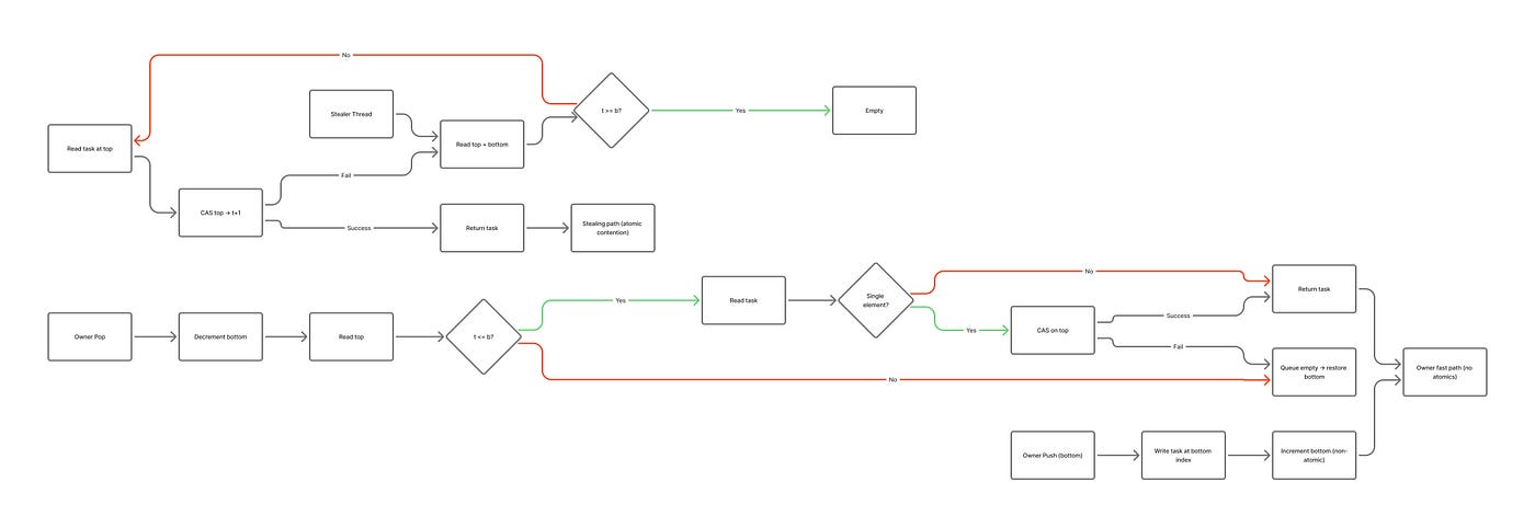
Every high-performance async executor uses work stealing. The data structure that makes it efficient is the Chase-Lev deque — a double-ended queue with asymmetric access: the owner accesses one end cheaply, stealers access the other end with atomic operations.

struct Deque<T>:
    buffer:  AtomicPtr<Buffer<T>>   // the backing circular array
    top:     AtomicI64              // stealers take from top — atomic
    bottom:  I64                    // owner pushes/pops from bottom — non-atomic locally

struct Buffer<T>:
    data:    T[]
    mask:    u64                    // capacity - 1

Owner push (called only by the owning thread):

push(task):
    b      = bottom
    t      = top.load(acquire)
    buf    = buffer.load(relaxed)

    if b - t >= buf.capacity - 1:
        grow()                      // resize — rare path
        buf = buffer.load(relaxed)

    buf.data[b & buf.mask] = task
    bottom = b + 1                  // non-atomic write — only owner writes bottom

Owner pop (also only called by the owning thread):

pop():
    b   = bottom - 1
    buf = buffer.load(relaxed)
    bottom = b                      // tentatively decrement

    t = top.load(seq_cst)           // seq_cst to synchronize with stealers
    if t <= b:
        task = buf.data[b & buf.mask]
        if t == b:                  // only one element — might race with a stealer
            if not top.compare_exchange(t, t+1, seq_cst, relaxed):
                bottom = b + 1     // stealer won — restore bottom, return empty
                return EMPTY
        return task
    else:
        bottom = b + 1             // queue was empty
        return EMPTY

Stealer (called by any other thread):

steal():
    loop:
        t   = top.load(acquire)
        b   = bottom.load(acquire)
        if t >= b: return EMPTY     // empty

        buf  = buffer.load(acquire)
        task = buf.data[t & buf.mask]

        if top.compare_exchange(t, t+1, seq_cst, relaxed):
            return task             // CAS succeeded — we got the task
        // CAS failed — another stealer got it, retry

The asymmetry is the key insight. The owner operates on bottom with non-atomic writes — no cache coherence traffic. Only the single-element edge case requires a CAS from the owner side. Stealers use CAS on top — they contend with each other but never with the owner except in the single-element case.

This means an executor thread running its own tasks pays essentially zero synchronization cost. The stealing path is more expensive, but stealing is rare — it only happens when a thread runs out of work.

Global Injection Queue — Task Entry Point

Newly spawned tasks and tasks woken from external threads (e.g., a waker called from an I/O driver thread) cannot go directly into a specific thread’s local deque — they do not know which thread is least loaded. They enter via a global injection queue.

The global queue is an MPSC (multiple producer, single consumer) or MPMC queue depending on whether multiple threads drain it:

struct GlobalQueue<T>:
    head: AtomicPtr<Node<T>>
    tail: AtomicPtr<Node<T>>

push(task):                          // called by any thread
    node = alloc Node(task, next=null)
    old_tail = tail.swap(node, acq_rel)
    old_tail.next.store(node, release)

steal_batch(local_deque, max_n):     // called by worker thread
    taken = 0
    while taken < max_n:
        node = pop_front()
        if node == null: break
        local_deque.push(node.task)
        taken++
    return taken

Workers check the global queue periodically — typically every N local pops (Tokio uses 61, a prime number to avoid alignment with other periodic operations). Taking a batch rather than a single task amortizes the cost of the global queue’s lock or CAS across multiple tasks.

LIFO Slot — Cache Locality Optimization

When a task spawns a child task and immediately awaits it, the child should run next — before anything else. The child will access data that the parent just touched, which is still hot in cache. Running the child immediately maximizes cache reuse.

Every worker thread has a single LIFO slot — a one-task buffer that bypasses the deque:

struct Worker:
    lifo_slot: AtomicOption<Task>
    local_deque: Deque<Task>

schedule(task):
    prev = lifo_slot.swap(Some(task), acq_rel)
    if prev is Some(old_task):
        local_deque.push(old_task)   // displaced task goes to normal queue

next_task():
    if let Some(task) = lifo_slot.take():
        return task                  // take LIFO slot first
    return local_deque.pop()
        or global_queue.steal()
        or steal_from_random_victim()

The spawning task puts the new task in the LIFO slot. On the next poll iteration, the worker picks it up immediately. The spawning task, now suspended waiting for the child, goes into the regular deque for later resumption.

This single optimization produces measurable throughput improvements for workloads with parent-child task relationships — which is most async workloads. Tokio calls this the “coop” optimization and measures 10–30% throughput improvement on typical HTTP server workloads.

Task Budget — Preventing Monopolization

A cooperative executor relies on tasks yielding control regularly. A task that never suspends (CPU-bound loop, very long synchronous operation) monopolizes the executor thread and starves all other tasks on that thread.

The budget mechanism gives each task a fixed number of “operations” per scheduling quantum:

struct TaskContext:
    budget: Cell<u8>             // decrements per operation, e.g. starts at 128

consume_budget(cx):
    b = cx.budget.get()
    if b == 0:
        cx.waker.wake_by_ref()   // re-schedule self
        return Pending           // yield to executor
    cx.budget.set(b - 1)
    return Continue

Each async I/O operation consumes one budget unit. When the budget reaches zero, the task schedules itself for resumption and yields — giving other tasks a chance to run. The task resumes on the next scheduler tick with a fresh budget.

This is why Tokio’s I/O operations are budget-aware — TcpStream::read internally calls consume_budget and may return Poll::Pending even when data is available, if the budget is exhausted. From the user's perspective the read "didn't complete yet" — from the scheduler's perspective, the task voluntarily yielded to prevent starvation.

Worker Parking — Efficient Idle

When all queues are empty, worker threads must sleep without burning CPU. The naive approach — thread::sleep(1ms) in a loop — burns CPU and introduces unnecessary latency. The correct approach is OS-level parking via futex (Linux) or equivalent.

struct Parker:
    state: AtomicU32             // EMPTY=0, PARKED=1, NOTIFIED=2

park():
    state.store(PARKED, release)
    loop:
        futex_wait(state, PARKED)   // blocks until state != PARKED
        if state.load(acquire) == NOTIFIED:
            state.store(EMPTY, release)
            return

unpark():
    old = state.swap(NOTIFIED, acq_rel)
    if old == PARKED:
        futex_wake(state, 1)        // wake one thread

The state machine prevents the lost wakeup race. If unpark is called between the worker's decision to park and the actual futex_wait call, the state is NOTIFIED — futex_wait returns immediately because the condition is already false.

Worker threads attempt to steal from all other threads before parking. The steal attempt itself serves as a final check for work before sleeping — prevents a scenario where a task is enqueued, the worker decides to park, the unpark is missed, and the task sits unexecuted.

6. Waker Internals and Notification

Atomic Waker — The Single-Slot Concurrent Waker

A future often needs to store a waker that will be replaced when the future is polled again. The naive approach — store the waker in a Mutex-protected Option — is correct but slow. The AtomicWaker uses a CAS-based state machine to avoid the mutex on the common path.

struct AtomicWaker:
    state: AtomicU8              // EMPTY=0, REGISTERING=1, WAKING=2, REGISTERED=3
    waker: UnsafeCell<Option<Waker>>

register(waker):
    loop:
        s = state.load(acquire)
        match s:
            EMPTY | REGISTERED:
                if state.compare_exchange(s, REGISTERING, acq_rel, acquire) succeeds:
                    waker_slot = waker
                    state.store(REGISTERED, release)
                    return

            WAKING:
                // concurrent wake — just call our waker directly
                waker.wake()
                return

wake():
    s = state.swap(WAKING, acq_rel)
    match s:
        REGISTERED:
            waker = take(waker_slot)
            state.store(EMPTY, release)
            waker.wake()

        REGISTERING:
            // register() is mid-flight — it will see WAKING state and self-wake
            // nothing to do here

        EMPTY | WAKING:
            // nothing registered, or already waking

The REGISTERING state prevents a race where register is mid-write when wake fires. The WAKING state prevents a race where wake fires mid-register. The state machine ensures exactly one of: the waker is called by wake(), or the registering thread sees WAKING and calls it itself. The invariant is: no wakeup is ever lost.

Poll-then-Register — The Correctness Protocol

The interaction between a future returning Pending and the waker being registered has a specific required ordering that must not be violated:

// WRONG — can miss events:
register_waker(cx.waker)          // register first
result = attempt_io()             // then try
if result == WOULD_BLOCK:
    return Pending
// Problem: event fired between register and attempt — attempt succeeded,
// but now we return Pending anyway. Task parks forever.

// ALSO WRONG — can miss wakeup:
result = attempt_io()             // try first
if result == WOULD_BLOCK:
    return Pending                // return Pending before registering waker
// Problem: event fires after attempt returns WOULD_BLOCK but before
// the caller registers the waker — wakeup is lost.

// CORRECT:
result = attempt_io()             // 1. try first
if result == WOULD_BLOCK:
    register_waker(cx.waker)      // 2. register
    result = attempt_io()         // 3. try again — closes the window
    if result == WOULD_BLOCK:
        return Pending            // 4. now safe — waker is registered
return Ready(result)

Step 3 is the critical addition. It closes the window between step 1 and step 2 where an event could fire and be missed. After step 2’s registration, any new event will call the waker and re-poll the future. If the event fired between steps 1 and 2, step 3 will succeed — the future returns Ready without parking.

7. Channel Internals

Slot Sequence Protocol — Dmitry Vyukov’s MPMC Queue

The highest-performance bounded MPMC (multiple producer multiple consumer) channel uses sequence numbers on each slot rather than locking the entire queue. This is the algorithm behind LMAX Disruptor, Rust’s crossbeam::ArrayQueue, and dozens of high-performance message queues.

struct Slot<T>:
    sequence: AtomicU64
    value:    UnsafeCell<T>

struct Queue<T>:
    slots:    Box<[Slot<T>]>     // fixed-size, cache-line padded
    head:     AtomicU64          // enqueue position
    tail:     AtomicU64          // dequeue position
    mask:     u64

// Initialization: slot[i].sequence = i for all i

Enqueue:

push(value):
    loop:
        pos  = head.load(relaxed)
        slot = slots[pos & mask]
        seq  = slot.sequence.load(acquire)
        diff = seq as i64 - pos as i64

        if diff == 0:
            // slot is ready for writing at this position
            if head.compare_exchange(pos, pos+1, relaxed, relaxed) succeeds:
                slot.value = value
                slot.sequence.store(pos + 1, release)  // signal slot is readable
                return Ok

        elif diff < 0:
            return Err(FULL)       // queue full

        // diff > 0 — another producer advanced head, retry with new pos

Dequeue:

pop():
    loop:
        pos  = tail.load(relaxed)
        slot = slots[pos & mask]
        seq  = slot.sequence.load(acquire)
        diff = seq as i64 - (pos + 1) as i64

        if diff == 0:
            // slot has data written for this position
            if tail.compare_exchange(pos, pos+1, relaxed, relaxed) succeeds:
                value = slot.value
                slot.sequence.store(pos + mask + 1, release)  // mark slot reusable
                return Ok(value)

        elif diff < 0:
            return Err(EMPTY)

        // another consumer advanced tail, retry

The sequence number eliminates the ABA problem entirely — it is a monotonically increasing counter, not a pointer, so it can never “wrap back” to a previous value within the useful lifetime of the queue. It also makes the algorithm wait-free on the fast path — no retry loop when there is no contention.

The release store after writing the value, paired with the acquire load of the sequence number by the consumer, ensures the value write is visible before the consumer reads it — without a full memory fence.

Async Park / Wake — The Channel Blocking Protocol

When a consumer finds the channel empty, it must park until a producer adds an item. The protocol must handle the race between “checking empty” and “going to sleep” — a producer may add an item between these two steps.

async fn recv(channel):
    loop:
        if let Some(value) = channel.try_pop():
            return value                    // fast path — no suspension

        waiter = Waiter(waker: cx.waker.clone(), value: None)
        channel.waiters.push(waiter_ptr)    // register intent to wait

        // critical: check again after registering
        if let Some(value) = channel.try_pop():
            channel.waiters.remove(waiter_ptr)
            return value                    // item arrived before we parked

        return Pending                      // safe to park — waker is registered

The second try_pop after registering the waiter closes the window. If a producer pushed between the first try_pop and the waiters.push, the item is in the queue and the second try_pop finds it. If the producer pushes after waiters.push, it will see the waiter and call its waker. Either way, no item is missed and no wakeup is lost.

On the producer side:

fn send(channel, value):
    channel.push(value)
    if let Some(waiter) = channel.waiters.pop():
        waiter.waker.wake()                 // wake one waiting consumer

The ordering is: push value first, then check waiters. This matches the consumer’s ordering: register waiter first, then check for value. This opposing ordering is what prevents the race — you cannot simultaneously miss both the value (consumer checks before push) and the waker (producer checks before registration).

8. Backpressure Algorithms

Token Bucket — Rate Limiting with Burst

The token bucket allows bursts up to a capacity while enforcing a long-term average rate. It is the correct algorithm for rate limiting async producers.

struct TokenBucket:
    tokens:       f64            // current token count
    capacity:     f64            // maximum tokens (burst size)
    refill_rate:  f64            // tokens per nanosecond
    last_refill:  Instant

acquire(cost):
    now = Instant::now()
    elapsed = now - last_refill
    tokens = min(capacity, tokens + elapsed * refill_rate)
    last_refill = now

    if tokens >= cost:
        tokens -= cost
        return Allow
    else:
        wait_time = (cost - tokens) / refill_rate
        return Deny(wait_time)    // caller may sleep wait_time and retry

The refill is lazy — tokens accumulate based on elapsed time, computed only when acquire is called. No background thread needed. This makes it efficient for async contexts where a background timer would require task spawning.

The burst capacity is what makes token bucket correct for network traffic: a connection that was idle for 1 second at a 1MB/s rate has banked 1MB of burst capacity. It can send 1MB immediately rather than being artificially throttled to 1KB/ms.

GCRA — Generic Cell Rate Algorithm

GCRA is mathematically equivalent to a token bucket but implemented with a single variable — the “theoretical arrival time” (TAT) of the next allowed request:

struct GCRA:
    tat:        AtomicU64        // theoretical arrival time, nanoseconds
    emission:   u64              // nanoseconds between emissions = 1/rate
    burst:      u64              // burst tolerance in nanoseconds = capacity/rate

check(cost_cells):
    increment = cost_cells * emission
    now       = current_time_ns()

    loop:
        old_tat = tat.load(acquire)
        new_tat = max(old_tat, now) + increment

        if new_tat - now > burst:
            wait = new_tat - increment - now + burst
            return Deny(wait)

        if tat.compare_exchange(old_tat, new_tat, acq_rel, acquire) succeeds:
            return Allow
        // CAS failed — another request updated tat concurrently, retry

GCRA’s advantage over token bucket in async contexts: the entire state is one 64-bit integer. The CAS makes it lock-free — multiple async tasks can check the rate limiter concurrently without a mutex. A token bucket with two fields (tokens + timestamp) requires two atomic updates, which cannot be done atomically together without a mutex or CAS on a 128-bit value.

Adaptive Concurrency Limiting — Little’s Law

Static concurrency limits (semaphores with fixed N) fail under variable load — too low means wasted capacity, too high means overload. Adaptive limiters use queuing theory to self-tune.

Little’s Law: L = λW — the average number of requests in the system equals the arrival rate times the average latency. Rearranging: λ = L / W — the maximum throughput equals concurrency divided by latency.

struct AdaptiveLimiter:
    limit:         AtomicU64       // current concurrency limit
    in_flight:     AtomicU64       // current in-flight requests
    min_rtt:       f64             // minimum observed round-trip time (no-load baseline)
    ewma_rtt:      f64             // smoothed current RTT

on_request_start():
    if in_flight.load() >= limit.load():
        return Reject

    in_flight.fetch_add(1)
    start_time = now()
    return Token(start_time)

on_request_end(token):
    rtt = now() - token.start_time
    in_flight.fetch_sub(1)

    ewma_rtt = alpha * rtt + (1-alpha) * ewma_rtt
    min_rtt  = min(min_rtt, rtt)   // decays slowly over time

    // Vegas algorithm: compute gradient
    gradient = 1.0 - (min_rtt / ewma_rtt)

    new_limit = limit * (1 + beta * gradient)
    new_limit = clamp(new_limit, min_limit, max_limit)
    limit.store(new_limit)

When ewma_rtt ≈ min_rtt: gradient ≈ 0 → limit holds steady — system is not overloaded. When ewma_rtt >> min_rtt: gradient → 1 → limit decreases — queuing is occurring, back off. When ewma_rtt improves: gradient becomes negative → limit increases — capacity available.

This self-tunes without any configuration. Netflix’s Concurrency Limiter, Google’s gRPC adaptive throttling, and Envoy’s adaptive concurrency filter all use variations of this approach.

9. Cancellation Internals

Two-Phase Cancel — The Correct Protocol

Cancellation has two distinct phases that must not be collapsed into one. Collapsing them creates races.

struct CancellationToken:
    state:     AtomicU8            // ALIVE=0, CANCELLING=1, CANCELLED=2
    callbacks: Mutex<List<Fn()>>   // registered cancel callbacks

// Phase 1: signal
cancel():
    if not state.compare_exchange(ALIVE, CANCELLING, acq_rel, acquire):
        return                     // already cancelled

    lock(callbacks.mutex)
    cbs = take(callbacks.list)
    unlock(callbacks.mutex)

    for cb in cbs:
        cb()                       // wake all registered waiters

    state.store(CANCELLED, release)

// Registration — must handle concurrent cancel
register(callback):
    lock(callbacks.mutex)
    if state.load(relaxed) == ALIVE:
        callbacks.list.push(callback)
        unlock(callbacks.mutex)
        return Registration(token_ptr, callback_ptr)
    else:
        unlock(callbacks.mutex)
        callback()                 // already cancelled — fire immediately
        return AlreadyCancelled

The lock on the callbacks list during both registration and the cancel flush is essential. Without it, a cancel that fires between the state check and the push in register would walk an empty list (missing the new callback) while register completes the push into a list nobody will ever walk again.

The two-phase state transition (ALIVE → CANCELLING → CANCELLED) allows in-flight operations to distinguish “cancel in progress” from “cancel complete” — useful for operations that must check whether cleanup is still necessary.

Cancellation Safety Analysis

Not every async operation is safe to cancel at every suspension point. The classification:

Cancellation-safe: operation can be dropped at any point without inconsistent state.

• Reading from a socket: data stays in kernel buffer, re-readable later
• A sleep/timer: timer simply never fires
• A pure computation with no side effects

Not cancellation-safe: dropping mid-operation leaves inconsistent state.

• Writing a framed message: may have written the header but not the body — peer receives corrupt stream
• A database transaction: may have executed some statements but not committed or rolled back
• A file write with fsync: may have written without syncing — data loss on crash

// Unsafe pattern:
async fn send_message(conn, msg):
    await conn.write(header(msg))    // SUSPEND POINT — if cancelled here,
    await conn.write(body(msg))      // body never sends — peer gets truncated message

// Safe pattern:
async fn send_message(conn, msg):
    buf = concat(header(msg), body(msg))
    await conn.write_all(buf)        // atomic from cancel perspective — one operation

The rule: an async operation is cancellation-safe if and only if the only observable effect of cancellation is “the operation did not complete” — not “the operation partially completed.” Partial completion is always worse than no completion because it leaves the system in an inconsistent state that is harder to recover from than a clean failure.

Structured concurrency enforces this discipline by making cancellation the default behavior when a scope exits — you are forced to reason about every operation’s cancellation safety upfront, not when debugging a production incident.

Conclusion

Modern async runtimes are not built on a single mechanism; they are the result of several carefully engineered layers working in concert. The event loop decides what runs next, the I/O backend determines when external work is ready, the promise and future machinery preserve compositional structure, coroutines preserve execution state across suspension points, and the scheduler ensures that all of it moves forward without wasting threads or violating fairness. Around these core pieces sit wakers, channels, backpressure controls, and cancellation protocols, each solving a specific failure mode that emerges under real load.

The important lesson is that async is not “magic parallelism.” It is a discipline of deferred execution. Every suspension point is a contractual boundary: state must be preserved, wakeups must not be lost, ordering must remain stable, and progress must be driven explicitly. When any one of those guarantees is violated, the result is not just slower code — it is incorrect code, often in subtle ways that only appear under contention, latency spikes, or cancellation races.

That is why understanding internals matters. A surface-level grasp of async/await is enough to write code that compiles, but not enough to write code that scales, remains responsive, and fails predictably. The real value of studying these internals is that it gives you a systems-level model: you can see where latency comes from, why tasks stall, how memory moves through the runtime, and which invariants must hold for the whole machine to stay correct.

In practice, this model changes how you debug and design. You stop treating hangs as mysteries and start tracing them back to missed wakeups, blocking work, queue pressure, or cancellation races. You stop treating performance issues as vague “async overhead” and start identifying whether the bottleneck is scheduling, I/O submission, timer churn, or contention in shared state. That shift — from abstraction to mechanism — is the difference between using async and understanding it.

If there is one overarching idea to keep, it is this: async runtimes do not eliminate complexity; they relocate it into explicit structures and rules. The abstraction is elegant because the machinery beneath it is strict. Once you understand that machinery, async code becomes far less magical and far more controllable.