How Text-to-Image Diffusion Models Work: The Full Pipeline

Type “a ferret reading a book by lantern light” into Stable Diffusion and, a few seconds later, it returns an image that did not previously exist. That output is produced by a pipeline of several networks, each with a narrow role. These components pass data from one stage to the next.

At the center of the pipeline is one model, the denoiser. It is trained on a single task: take an image with random Gaussian noise added to it — and estimate that noise so it can be subtracted, yielding a slightly cleaner image. A network that reliably removes a small amount of noise can be applied repeatedly: starting from pure noise and denoising in small steps, dozens or hundreds of times, converts random noise into a coherent image. The prompt is supplied to the denoiser as an additional input at every step, steering which image the noise resolves toward, so the output matches the text. The other components exist to support this loop — encoding the prompt, compressing the image, and scheduling how much noise is removed at each step.

How an image is generated

Before introducing formulas, here is the inference process in plain terms.

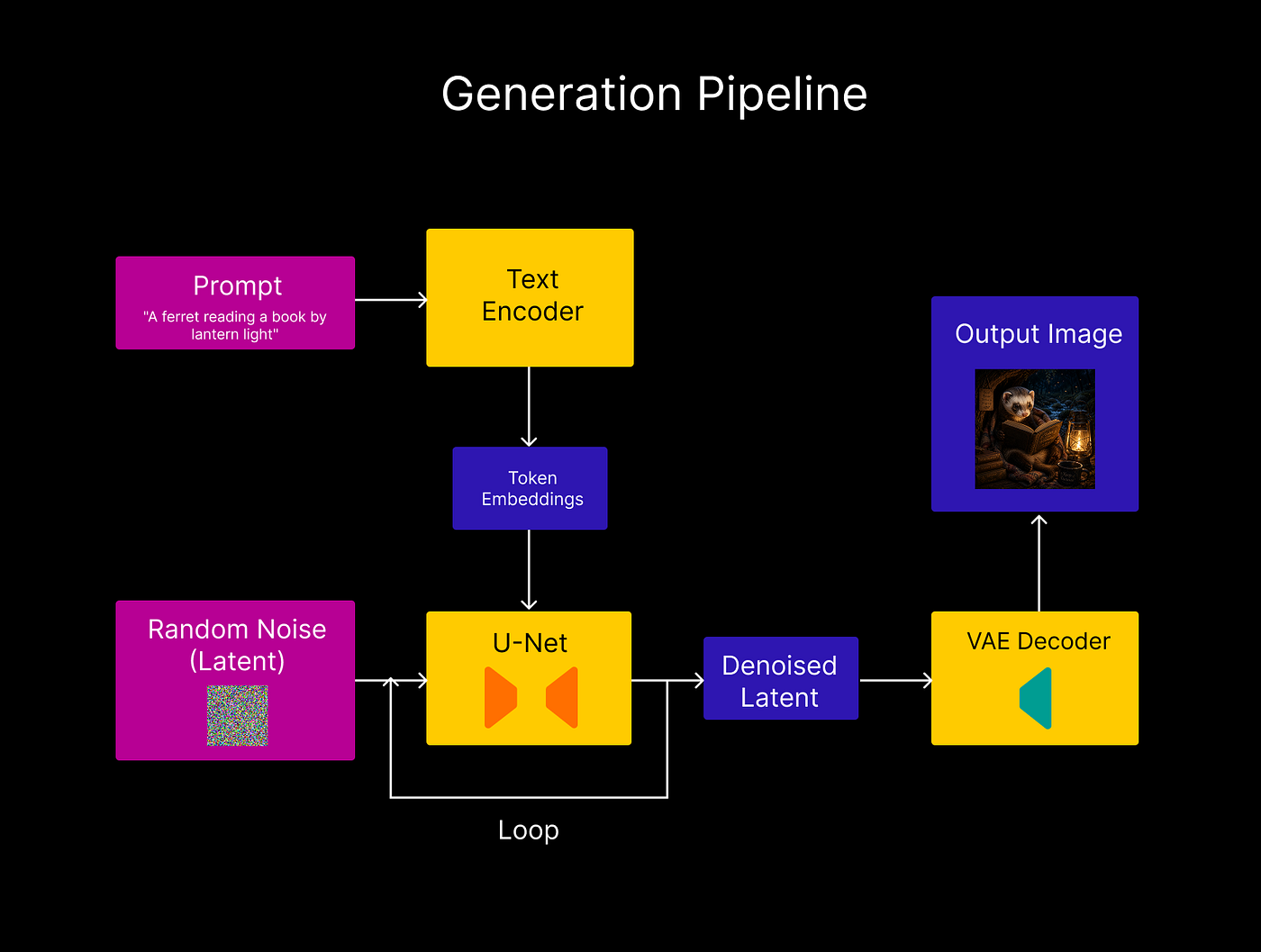
Everything starts with the prompt. The text encoder reads it and converts it into a sequence of embedding vectors that encode its meaning; for the rest of the pipeline, “a ferret reading a book by lantern light” is represented solely by these embeddings.

In parallel, the system samples a small array of pure random (Gaussian) noise. This array is the starting point for the image and initially carries no information about the prompt.

The U-Net then runs. It takes the noisy array together with the encoded prompt and removes a small amount of the noise, conditioned on the text. A single pass removes only a little, so the process repeats: the slightly cleaner array is fed back into the U-Net dozens of times. Across passes, coarse structure appears first and fine detail later. The scheduler controls the loop, setting exactly how much noise is removed at each step so the sequence converges to a clean result.

One key efficiency point: all of this runs on a small, compressed representation of the image, which keeps each pass cheap. When the loop finishes, the VAE decoder maps the final latent back to a full-resolution image.

That is the complete process. The rest of the post adds precision: what each component does internally, the relevant formulas, and how each part is trained.

Component 1: the text encoder (CLIP)

A Transformer (CLIP’s text tower in Stable Diffusion 1.x) turns the tokenized prompt into a matrix of embeddings of shape L × d: the prompt is padded or truncated to L tokens, and each token is mapped to a d-dimensional embedding vector. CLIP was pre-trained on hundreds of millions of image–caption pairs to place matching images and texts close together in a shared vector space, so its embeddings already encode visual meaning. It is frozen during diffusion training.

What CLIP is trained on

CLIP is trained first, on a contrastive task that is entirely separate from diffusion. The inputs are (image, caption) pairs. Two networks are trained jointly: an image encoder maps each image to a single pooled embedding, and the text encoder maps each caption to a single pooled embedding (the hidden state at the end-of-sequence token), both in a shared vector space. The contrastive loss pulls each image embedding toward the embedding of its own caption and pushes it away from all other captions in the batch. After enough pairs, the embedding of “a photo of a ferret” and the embedding of an actual photo of a ferret lie close together in that space, so the text embeddings encode visual content.

Component 2: the VAE

Why work in a latent space at all? For a picture of size H × W with three color channels, the pixel representation has 3·H·W values, and running a large network over all of them dozens of times is expensive. The VAE encoder compresses the image by a factor of f per side into a latent of shape M × N × c, where N = H/f, M = W/f, and c is a small number of channels — far fewer values overall. All of the expensive diffusion computation happens in this latent space, and only at the end does the VAE decoder map the result back to pixels.

How the VAE is trained

In the conceptual training sequence, the VAE is trained before the UNet, because the UNet depends on a fixed latent space. The VAE is trained on images alone — captions play no role here. The full autoencoder runs end to end, but note the “variational” detail: the encoder does not output a latent directly. It outputs the parameters of a Gaussian over the latent — a mean and a log-variance per latent dimension — and a latent z is then sampled from that distribution. The decoder reconstructs the image from z, and the output is compared against the input.

This stage defines the latent space everything else operates in, which is why it must finish before U-Net training begins: if the latent space kept changing, the U-Net’s target would be non-stationary.

Component 3: the U-Net

The U-Net is the only network trained for diffusion itself. It has the characteristic U shape: a downsampling path that reduces spatial resolution while extracting features, a bottleneck, and an upsampling path that restores resolution, with skip connections passing features from each down level to its matching up level.

The timestep t enters as a sinusoidal embedding added inside every block, so the network knows the current noise level. The text enters through cross-attention layers, which warrant a closer look.

What the U-Net receives from the text encoder

This full L × d sequence of per-token hidden states — the output of CLIP’s final layer, one vector per token — is exactly what the U-Net’s cross-attention layers consume, as the keys and values. The pipeline does not collapse the prompt to a single vector; every token’s embedding is passed through, which is what lets different image regions attend to different words.

The query (Q) comes from the image. Inside the U-Net, the image is a feature tensor of shape (h, w, c): a grid of h × w spatial positions, each holding a vector of c channel values. For a position (i, j), that c-dimensional vector summarizes what is currently represented at that location. A learned matrix Wq projects it into a query. The full grid therefore produces h·w queries — one per position.

The keys (K) come from the text. A second learned matrix Wk projects each of the L token embeddings into a key vector, encoding what that token represents. Keys are compared against queries.

The values (V) also come from the text. A third learned matrix Wv maps every token to a value vector — the content the token contributes: the textures, shapes, and colors associated with it. Keys determine how strongly each token is attended to; values determine the content that token contributes.

Note the asymmetry between the two: CLIP’s contrastive objective is defined on the single pooled embedding per caption, but diffusion discards that pooled vector and instead uses the full per-token sequence from CLIP’s final layer.

How it’s trained

With CLIP and the VAE frozen, training optimizes a single objective: given a noisy latent, the timestep, and the text, predict the noise that was added.

Step by step: the image passes through the frozen VAE encoder to produce a clean latent z₀. The caption passes through the frozen text encoder to produce embeddings c.

The scheduler samples a random timestep t between 1 and T (the total number of noise levels), samples Gaussian noise ε, and mixes it into the latent:

Here ᾱₜ is a value between 0 and 1 from a fixed table: at small t the latent is barely noisy, at large t it is nearly pure noise.

The U-Net receives noised latent zₜ, timestamp t, and text embedding c, and predicts the noise. The loss is mean squared error:

That is the entire training objective — a single regression task: predict the noise.

One detail in the data: roughly 10% of the time the caption is replaced with an empty prompt, so the same U-Net also learns to denoise unconditionally — the prerequisite for classifier-free guidance at inference.

The training sequence

Stepping back, the system is built in a fixed order, one component at a time. CLIP is trained first, on its own contrastive task over image–caption pairs, then frozen. The VAE is trained second, on images alone, to compress and reconstruct them; freezing it fixes the latent space everything else depends on. The U-Net is trained third — the main training run — to predict the noise added to a frozen VAE’s latents, conditioned on frozen CLIP’s text embeddings. Optional fine-tuning comes last (full fine-tuning, LoRA, DreamBooth, ControlNet), centered on the U-Net but often also touching the text encoder, with the VAE left frozen. The scheduler is not a neural network and is not trained; it follows a fixed noise schedule and update rule.

The inference-time pipeline

Generation runs the process in reverse: starting from pure random noise, the U-Net progressively denoises it, conditioned on the text.

The prompt is encoded once into embeddings c. The starting latent is sampled as pure Gaussian noise. The loop then runs, typically 30–50 times: the U-Net predicts the noise in the current latent, and the scheduler uses that prediction to compute a slightly cleaner latent. After the final step, the VAE decoder maps the clean latent to the final image. At inference time, the VAE is used only as a decoder, and the text encoder runs once per prompt.

One important addition: classifier-free guidance (CFG). At each step the U-Net runs twice — once with the prompt and once with an empty prompt — and the two predictions are combined:

The guidance scale s amplifies the direction toward the prompt, which strengthens how closely the image follows the text. This is what the caption dropout during training enables: because the same U-Net learned both conditional and unconditional denoising, it can produce both predictions here.

Conclusion

A text-to-image diffusion model combines several components, each with a clear role. The text encoder converts the prompt into vectors, the VAE bridges pixel space and a compact latent space, the scheduler meters noise in and out, and the U-Net — the only component trained for diffusion — is optimized for a single task: predicting noise. Applied iteratively, starting from random noise and conditioned on text through cross-attention and classifier-free guidance, the pipeline can generate an image for an arbitrary text prompt.

Links & References

Denoising Diffusion Probabilistic Models (Ho et al., 2020) — the DDPM paper that established the noise-prediction training objective.

High-Resolution Image Synthesis with Latent Diffusion Models (Rombach et al., 2022) — the Stable Diffusion paper; introduces doing diffusion in VAE latent space.

Learning Transferable Visual Models From Natural Language Supervision (Radford et al., 2021) — the CLIP paper behind the text encoder.

Classifier-Free Diffusion Guidance (Ho & Salimans, 2022) — the method that makes prompts effectively steer the image.

Hugging Face Diffusers documentation — implementation code for every component discussed here.