Using Hidden Markov Models to Read Stock Market Regimes

Why I Use HMM as a Stock Research Tool

Photo by Emily Morter on Unsplash

A stock chart looks like one continuous price line, but the market behind that line is not always operating under the same condition. Apple can spend one month in a calm upward drift, another month in a noisy sideways structure, and another period under volatility pressure. If we force all those days into one average return and one volatility number, we lose the structure that actually matters.

This is where a Hidden Markov Model, or HMM, becomes useful. I do not treat it as a magic price predictor. The better use is more modest: HMM can help label the current price environment. It can answer a practical question:

What kind of state does this stock look like right now?

That question is useful before doing deeper research. It helps separate a strong recent structure from a stressed one. It also gives a neutral label when the stock is neither breaking down nor showing strong momentum.

The experiment below uses AAPL as a single-stock example. The same idea can later be expanded into a stock scanner that classifies thousands of tickers and builds candidate pools such as a “recent strong-structure Top 500.” The uploaded single-stock script uses a wide adjusted-close CSV, computes return, volatility, momentum, drawdown, market return, and relative return features, then fits a three-state Gaussian HMM to AAPL.

Hidden Markov Model

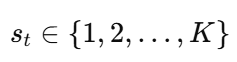
An HMM assumes that the data we observe is generated by hidden states. In stock research, the observed data may be daily return, rolling volatility, momentum, and drawdown. The hidden state may be something like “bullish recovery”, “neutral structure”, or “bearish stress”.

Mathematically, the hidden state at time t is:

The observed feature vector is:

A Gaussian HMM assumes:

This means each state has its own mean vector and covariance matrix. A bullish state may have better returns, stronger momentum, and smaller drawdown. A stress state may have weaker returns, higher volatility, and deeper drawdown. The neutral state usually sits somewhere in between.

The state sequence follows a Markov transition rule:

All transition probabilities form the transition matrix:

The key idea is not complicated. Today’s hidden state depends on yesterday’s hidden state, and today’s observed market features depend on today’s hidden state. The HMM memo describes this structure as a model that learns hidden states, transition behavior, state probabilities, and the most likely state path from observed stock features.

Data Used in the AAPL Example

The single-stock experiment uses a wide adjusted-close price table. The expected structure is simple:

Date, AAPL, MSFT, NVDA, SPY, QQQ, ...
2020-01-02, ...
2020-01-03, ...

Each row is one trading day. Each ticker is one column. AAPL is the target stock. The other tickers can be used to estimate a rough market return. In this version, market return is calculated as the equal-weight average log return of all usable non-AAPL columns.

The AAPL feature set contains:

ret          daily log return
rv5          5-day rolling volatility
rv20         20-day rolling volatility
mom5         5-day log momentum
mom20        20-day log momentum
drawdown20   distance from 20-day rolling high
mkt_ret      broad market average log return
mkt_rv20     20-day market volatility
rel_ret      AAPL return minus market return

This design matters. If the model only sees returns, it may miss the difference between a low-volatility drift and a high-volatility bounce. Momentum and drawdown add price-structure information. Market return and relative return help separate stock-specific behavior from broad market movement.

Practical Python Code for One Stock

The following code is a compact version of the AAPL experiment. It is written for a local CSV file with adjusted close prices in wide format. It fits a three-state Gaussian HMM, prints the transition matrix, estimates state durations, labels states, and saves three CSV files: state probabilities, state summary, and transition matrix.

import os
import numpy as np
import pandas as pd
from hmmlearn.hmm import GaussianHMM
from sklearn.preprocessing import StandardScaler

CSV_PATH = "prices_adjclose_wide.csv"
TICKER = "AAPL"
N_STATES = 3
RANDOM_STATE = 42
OUT_DIR = r"C:\ai_stock_platform"

def build_single_ticker_features(prices_wide: pd.DataFrame, ticker: str) -> pd.DataFrame:
    df = prices_wide.copy()
    df["Date"] = pd.to_datetime(df["Date"])
    df = df.sort_values("Date").reset_index(drop=True)

    if ticker not in df.columns:
        raise ValueError(f"{ticker} not found in CSV columns.")

    px = pd.to_numeric(df[ticker], errors="coerce")
    out = pd.DataFrame({"Date": df["Date"], "Close": px})

    out["ret"] = np.log(out["Close"] / out["Close"].shift(1))
    out["rv5"] = out["ret"].rolling(5).std()
    out["rv20"] = out["ret"].rolling(20).std()
    out["mom5"] = np.log(out["Close"] / out["Close"].shift(5))
    out["mom20"] = np.log(out["Close"] / out["Close"].shift(20))
    out["drawdown20"] = out["Close"] / out["Close"].rolling(20).max() - 1.0

    market_cols = [c for c in df.columns if c not in ["Date", ticker]]
    market = df[market_cols].apply(pd.to_numeric, errors="coerce")
    market_ret = np.log(market / market.shift(1)).mean(axis=1, skipna=True)

    out["mkt_ret"] = market_ret
    out["mkt_rv20"] = out["mkt_ret"].rolling(20).std()
    out["rel_ret"] = out["ret"] - out["mkt_ret"]

    out = out.replace([np.inf, -np.inf], np.nan)
    return out.dropna().reset_index(drop=True)

def fit_hmm(feat: pd.DataFrame, n_states: int = 3):
    feature_cols = [
        "ret", "rv5", "rv20",
        "mom5", "mom20",
        "drawdown20",
        "mkt_ret", "mkt_rv20", "rel_ret"
    ]

    X = feat[feature_cols].values

    scaler = StandardScaler()
    X_std = scaler.fit_transform(X)

    hmm = GaussianHMM(
        n_components=n_states,
        covariance_type="full",
        n_iter=300,
        random_state=RANDOM_STATE
    )

    hmm.fit(X_std)

    result = feat.copy()
    result["state_viterbi"] = hmm.predict(X_std)

    state_prob = hmm.predict_proba(X_std)
    for k in range(n_states):
        result[f"p_state_{k}"] = state_prob[:, k]

    return result, hmm, feature_cols

def summarize_states(result: pd.DataFrame, hmm: GaussianHMM) -> pd.DataFrame:
    summary = (
        result.groupby("state_viterbi")
        .agg(
            n_days=("ret", "size"),
            avg_ret=("ret", "mean"),
            vol_ret=("ret", "std"),
            avg_rv20=("rv20", "mean"),
            avg_mom20=("mom20", "mean"),
            avg_drawdown20=("drawdown20", "mean"),
            avg_rel_ret=("rel_ret", "mean"),
        )
        .reset_index()
    )

    A = hmm.transmat_
    expected_duration = 1.0 / (1.0 - np.diag(A))

    duration_df = pd.DataFrame({
        "state_viterbi": np.arange(hmm.n_components),
        "self_transition_prob": np.diag(A),
        "expected_duration_days": expected_duration
    })

    return summary.merge(duration_df, on="state_viterbi", how="left")

def label_states(summary: pd.DataFrame) -> pd.DataFrame:
    summary = summary.copy()
    summary["state_label"] = "neutral_or_mixed"

    best_ret_state = summary["avg_ret"].idxmax()
    worst_ret_state = summary["avg_ret"].idxmin()
    highest_vol_state = summary["vol_ret"].idxmax()

    summary.loc[best_ret_state, "state_label"] = "bullish_or_recovery"
    summary.loc[worst_ret_state, "state_label"] = "bearish_or_stress"

    if highest_vol_state not in [best_ret_state, worst_ret_state]:
        summary.loc[highest_vol_state, "state_label"] = "high_volatility"

    return summary

def main():
    os.makedirs(OUT_DIR, exist_ok=True)

    raw = pd.read_csv(CSV_PATH)
    feat = build_single_ticker_features(raw, TICKER)

    result, hmm, feature_cols = fit_hmm(feat, N_STATES)
    summary = label_states(summarize_states(result, hmm))

    A = hmm.transmat_
    expected_duration = 1.0 / (1.0 - np.diag(A))

    print("Ticker:", TICKER)
    print("Feature columns:", feature_cols)
    print("Transition matrix:\n", A)
    print("Expected durations in trading days:\n", expected_duration)
    print("\nState summary:\n", summary)

    prob_cols = [f"p_state_{k}" for k in range(N_STATES)]
    print("\nLatest rows:\n")
    print(result[["Date", "Close", "state_viterbi"] + prob_cols].tail(10))

    result.to_csv(os.path.join(OUT_DIR, f"hmm_state_probs_{TICKER}.csv"), index=False)
    summary.to_csv(os.path.join(OUT_DIR, f"hmm_state_summary_{TICKER}.csv"), index=False)
    pd.DataFrame(A).to_csv(os.path.join(OUT_DIR, f"hmm_transition_matrix_{TICKER}.csv"), index=False)

if __name__ == "__main__":
    main()

The uploaded single-stock file follows the same practical structure: build AAPL features, standardize them, fit GaussianHMM, predict Viterbi states, compute state probabilities, summarize states, label regimes, and save output files.

Understanding the AAPL Output

The AAPL run used these feature columns:

ret, rv5, rv20, mom5, mom20, drawdown20, mkt_ret, mkt_rv20, rel_ret

The fitted transition matrix was:

[[0.86469903 0.09339726 0.04190371]
 [0.02003538 0.95423632 0.02572830]
 [0.02999262 0.00904774 0.96095964]]

The diagonal values tell us how sticky each state is. State 0 has a self-transition probability of about 0.865. State 1 is more persistent at about 0.954. State 2 is even slightly more persistent at about 0.961.

Expected duration is calculated as:

The AAPL output produced:

State 0:  7.39 trading days
State 1: 21.85 trading days
State 2: 25.61 trading days

After state labeling, the model interpreted the states as:

State 0: bullish_or_recovery
State 1: neutral_or_mixed
State 2: bearish_or_stress

The state summary counted 391 days in state 0, 1,012 days in state 1, and 1,091 days in state 2. The large count in the stress state does not mean Apple was “bad” for 1,091 days. It means that, under this feature set and label rule, many historical observations had the statistical profile of the weakest-return regime.

The latest rows are the most useful part for daily research. On 2025–09–29, AAPL had a state 1 probability around 0.9987. On 2025–09–30, state 1 probability was almost 1.0000. On 2025–10–02, state 1 probability was still around 0.9994, while state 2 probability was only about 0.0005.

That is a clear result. AAPL was classified as neutral or mixed, not bullish recovery and not bearish stress. The model was not giving a buy signal. It was saying: recent AAPL price behavior looked stable, but not strongly bullish under the selected features.

For a stock researcher, this is useful. AAPL can be kept in the research universe as a non-stressed mega-cap, while stronger momentum candidates may be found elsewhere.

Scaling the Idea Into a Stock Scanner

The same HMM logic can be expanded from one stock to a full stock universe. The end-to-end scanner in the uploaded files produces three main outputs: current price-state labels, recent strong-structure Top 500, and a stress/risk review list. It also clearly says these outputs are not buy/sell signals. They are unsupervised structure outputs.

The “current state label” output is the simplest one. Every valid ticker receives a label such as:

bullish_or_recovery
neutral_or_mixed
bearish_or_stress

The “recent strong-structure Top 500” is more interesting. It is not a prediction list. It is a candidate pool. The scanner combines bullish probability, low stress probability, 20-day momentum, relative return, shallow drawdown, and controlled volatility. The result is a ranked universe of stocks with strong recent price structure.

That kind of list is useful at the beginning of research. A human analyst can then study fundamentals, industry trend, earnings quality, valuation, liquidity, and catalysts. HMM helps reduce the universe from thousands of tickers to a more focused research sample.

The stress list serves the opposite function. It highlights stocks that currently look weak or stressed under the HMM state model. A stress label should not trigger automatic selling, but it should trigger review. If a stock has high stress probability, weak relative return, large drawdown, and high volatility, I want to know that before adding capital.

Suggestions

A three-state HMM is a good starting point. Two states may be too rough, while five or six states can become difficult to interpret. A simple structure with bullish/recovery, neutral/mixed, and bearish/stress is usually enough for screening.

Feature design is more important than model complexity. Return alone is not enough. Volatility, momentum, drawdown, market return, and relative return give the model a better view of price structure.

The state labels should be treated as economic interpretations, not mathematical truth. HMM state numbers are arbitrary. State 0 has no built-in meaning until we inspect its return, volatility, momentum, and drawdown profile.

The model should not be used alone for trading. The scanner documentation makes this boundary clear: HMM is useful for state identification, recent strength classification, and risk-background scanning, but not reliable enough as a direct trading signal.

Conclusion

HMM is valuable in stock research because it gives structure to noisy price data. It can label AAPL as neutral, identify a strong-structure stock universe, and produce a stress review list for risk control.

The method does not replace valuation, industry research, or portfolio judgment. Its strength is earlier in the workflow. It helps decide where to look first.

That is already enough. In practical stock research, a tool that improves sample selection can be more useful than a model pretending to predict tomorrow’s price.

About me

With over 20 years of experience in software and database management and 25 years teaching IT, math, and statistics, I am a Data Scientist with extensive expertise across multiple industries.

You can connect with me at:

Email: datalev@gmail.com | LinkedIn | https://shenggang.substack.com