ARIMA Implementation: From Theory to Production-Ready Forecasts

Part 6 of 8: ARIMA Models Part 2 — Building, Diagnosing, and Forecasting

Welcome back! In Part 5, we learned the theory: AR, MA, ACF/PACF patterns, and how to identify models. Rachel understood what ARIMA is, but she still needed to know how to build one.

Today, we’re going from theory to code. By the end of this article, you’ll have production-ready ARIMA models.

It’s Wednesday. Rachel has identified that her exchange rate data needs ARIMA(1,1,1) based on ACF/PACF plots. She opens Python. Now what?

“How do I actually fit this model?” “What if my (p,d,q) guess is wrong?” “How do I know if the model is good?” “How do I generate forecasts with confidence intervals?”

This is Part 6: Implementation. Let’s build.

Setup: Tools and Data

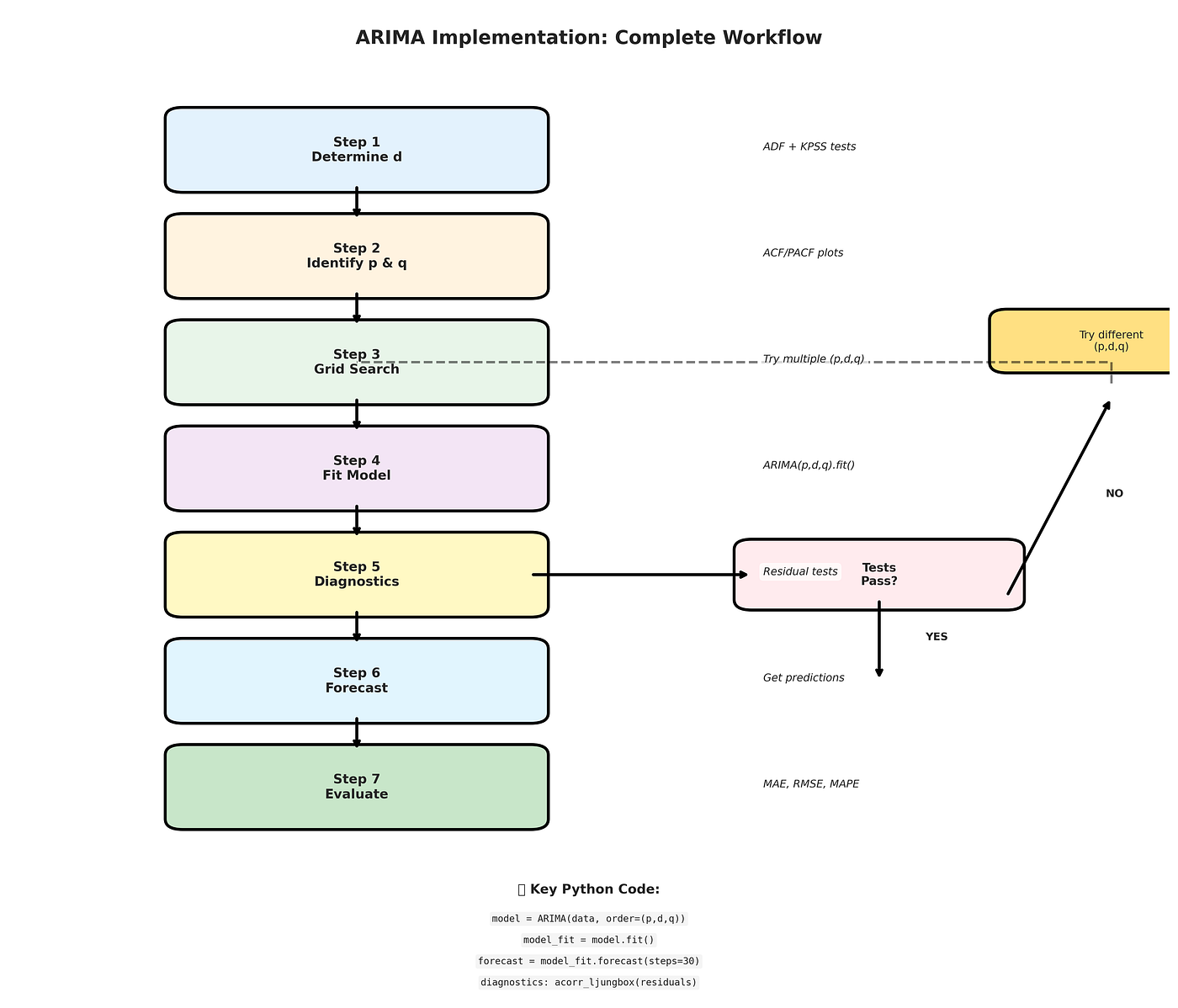
Figure 1: Complete ARIMA implementation workflow. Follow these 7 steps from determining d to evaluating forecasts.

import pandas as pd
import numpy as np
import matplotlib.pyplot as plt
import seaborn as sns
from statsmodels.tsa.stattools import adfuller, kpss, acf, pacf
from statsmodels.graphics.tsaplots import plot_acf, plot_pacf
from statsmodels.tsa.arima.model import ARIMA
from statsmodels.stats.diagnostic import acorr_ljungbox
from scipy import stats
import warnings
warnings.filterwarnings('ignore')

# Set style
sns.set_style("whitegrid")
plt.rcParams['figure.figsize'] = (16, 10)

np.random.seed(42)

print("ARIMA Implementation - Part 6")
print("="*60)

Let’s use real-world-like data: daily stock returns.

# Generate realistic stock price data
n = 500
dates = pd.date_range('2020-01-01', periods=n, freq='D')

# Random walk with drift (common for stock prices)
drift = 0.0005
innovations = np.random.normal(0, 0.02, n)
log_returns = drift + innovations
prices = 100 * np.exp(np.cumsum(log_returns))

# Create DataFrame
df = pd.DataFrame({
    'price': prices,
    'returns': log_returns
}, index=dates)

print(f"\nData shape: {df.shape}")
print(f"Date range: {df.index.min()} to {df.index.max()}")
print("\nFirst few rows:")
print(df.head())

# Quick visualization
fig, axes = plt.subplots(2, 1, figsize=(16, 8))

axes[0].plot(df.index, df['price'], linewidth=1.5, color='#2E86AB')
axes[0].set_title('Stock Price (Non-Stationary)', fontsize=13, fontweight='bold')
axes[0].set_ylabel('Price ($)')
axes[0].grid(True, alpha=0.3)

axes[1].plot(df.index, df['returns'], linewidth=1, color='#06A77D', alpha=0.8)
axes[1].axhline(y=0, color='red', linestyle='--', alpha=0.3)
axes[1].set_title('Returns (Stationary)', fontsize=13, fontweight='bold')
axes[1].set_ylabel('Returns')
axes[1].set_xlabel('Date')
axes[1].grid(True, alpha=0.3)

plt.tight_layout()
plt.savefig('stock_data_overview.png', dpi=300, bbox_inches='tight')
plt.show()

Step 1: Determine d (Order of Differencing)

From Part 3, we know how to test stationarity. Let’s be systematic.

def determine_differencing_order(series, max_d=2):
    """
    Determine optimal differencing order using ADF and KPSS tests

    Returns:
    --------
    d : int
        Recommended differencing order
    """
    print("\n" + "="*60)
    print("DETERMINING DIFFERENCING ORDER (d)")
    print("="*60)

    current_series = series.copy()

    for d in range(max_d + 1):
        print(f"\n--- Testing d={d} ---")

        # ADF test (H0: non-stationary)
        adf_result = adfuller(current_series.dropna())
        adf_stat = adf_result[1]

        # KPSS test (H0: stationary)
        kpss_result = kpss(current_series.dropna(), regression='c')
        kpss_stat = kpss_result[1]

        print(f"ADF p-value:  {adf_stat:.6f} {'✓ Stationary' if adf_stat < 0.05 else '✗ Non-stationary'}")
        print(f"KPSS p-value: {kpss_stat:.6f} {'✓ Stationary' if kpss_stat > 0.05 else '✗ Non-stationary'}")

        # Both tests agree it's stationary
        if adf_stat < 0.05 and kpss_stat > 0.05:
            print(f"\n✅ RESULT: Use d={d}")
            return d

        # Try next difference
        if d < max_d:
            current_series = current_series.diff().dropna()
            print(f"→ Taking difference {d+1}...")

    print(f"\n⚠️  WARNING: Even d={max_d} not clearly stationary. Using d={max_d}")
    return max_d

# Test on prices (should need d=1)
d_price = determine_differencing_order(df['price'])

# Test on returns (should need d=0)
d_returns = determine_differencing_order(df['returns'])

Result: Prices need d=1, returns need d=0. We’ll work with returns (already stationary).

Step 2: Identify p and q Using ACF/PACF

def identify_arima_orders(series, max_lags=40):
    """
    Plot ACF and PACF to help identify p and q

    Interpretation guide:
    - ACF cuts off at q, PACF decays → MA(q)
    - ACF decays, PACF cuts off at p → AR(p)
    - Both decay → ARMA(p,q)
    """
    print("\n" + "="*60)
    print("IDENTIFYING p AND q USING ACF/PACF")
    print("="*60)

    fig, axes = plt.subplots(1, 2, figsize=(16, 5))

    # ACF
    plot_acf(series.dropna(), lags=max_lags, ax=axes[0])
    axes[0].set_title('Autocorrelation Function (ACF)', fontsize=13, fontweight='bold')
    axes[0].set_xlabel('Lag')

    # PACF
    plot_pacf(series.dropna(), lags=max_lags, ax=axes[1], method='ywm')
    axes[1].set_title('Partial Autocorrelation Function (PACF)', fontsize=13, fontweight='bold')
    axes[1].set_xlabel('Lag')

    plt.tight_layout()
    plt.savefig('acf_pacf_analysis.png', dpi=300, bbox_inches='tight')
    plt.show()

    # Count significant lags
    acf_values = acf(series.dropna(), nlags=max_lags)
    pacf_values = pacf(series.dropna(), nlags=max_lags, method='ywm')

    # Significance threshold (95% confidence)
    n = len(series.dropna())
    threshold = 1.96 / np.sqrt(n)

    # Find where ACF cuts off (first becomes insignificant)
    acf_cutoff = 0
    for i in range(1, len(acf_values)):
        if abs(acf_values[i]) > threshold:
            acf_cutoff = i
        else:
            break

    # Find where PACF cuts off
    pacf_cutoff = 0
    for i in range(1, len(pacf_values)):
        if abs(pacf_values[i]) > threshold:
            pacf_cutoff = i
        else:
            break

    print(f"\nACF significant up to lag: {acf_cutoff}")
    print(f"PACF significant up to lag: {pacf_cutoff}")

    print("\n📊 Interpretation Guide:")
    if acf_cutoff <= 2 and pacf_cutoff > 5:
        print(f"→ ACF cuts off early, PACF decays → Try MA({acf_cutoff})")
        suggested_models = [(0, 0, acf_cutoff), (0, 0, acf_cutoff+1)]
    elif pacf_cutoff <= 2 and acf_cutoff > 5:
        print(f"→ PACF cuts off early, ACF decays → Try AR({pacf_cutoff})")
        suggested_models = [(pacf_cutoff, 0, 0), (pacf_cutoff+1, 0, 0)]
    else:
        print(f"→ Both decay → Try ARMA({min(pacf_cutoff, 2)}, {min(acf_cutoff, 2)})")
        suggested_models = [(1, 0, 1), (2, 0, 1), (1, 0, 2)]

    print(f"\n💡 Suggested models to try: {suggested_models}")

    return suggested_models

# Identify orders for returns
suggested = identify_arima_orders(df['returns'])

Step 3: Fit ARIMA Models

Now comes the actual modeling. Let’s fit multiple candidates and compare.

def fit_arima_model(series, order, seasonal_order=None):
    """
    Fit ARIMA model and return results

    Parameters:
    -----------
    series : pd.Series
        Time series data
    order : tuple
        (p, d, q) for ARIMA
    seasonal_order : tuple, optional
        (P, D, Q, s) for SARIMA

    Returns:
    --------
    model_fit : ARIMAResults
        Fitted model
    """
    try:
        if seasonal_order:
            model = ARIMA(series, order=order, seasonal_order=seasonal_order)
        else:
            model = ARIMA(series, order=order)

        model_fit = model.fit()
        return model_fit

    except Exception as e:
        print(f"Error fitting ARIMA{order}: {e}")
        return None

# Fit our first model: ARIMA(1,0,1) on returns
print("\n" + "="*60)
print("FITTING ARIMA(1,0,1)")
print("="*60)

model_fit = fit_arima_model(df['returns'], order=(1, 0, 1))

if model_fit:
    print("\n✅ Model fitted successfully!")
    print("\nModel Summary:")
    print(model_fit.summary())

Step 4: Model Diagnostics

Figure 2: Four critical diagnostic tests for ARIMA models. Pass at least 3 tests for an adequate model.

Critical: Never trust a model without diagnostics!

def diagnose_arima_model(model_fit, series_name="Series"):
    """
    Comprehensive ARIMA model diagnostics

    Checks:
    1. Residuals look like white noise
    2. No autocorrelation in residuals
    3. Residuals are normally distributed
    4. No heteroskedasticity
    """
    print("\n" + "="*60)
    print(f"DIAGNOSTIC TESTS FOR {series_name}")
    print("="*60)

    residuals = model_fit.resid

    # Create diagnostic plots
    fig, axes = plt.subplots(2, 3, figsize=(16, 10))
    fig.suptitle(f'ARIMA Diagnostic Plots: {series_name}', fontsize=16, fontweight='bold')

    # 1. Residuals over time
    axes[0, 0].plot(residuals, linewidth=1, alpha=0.8)
    axes[0, 0].axhline(y=0, color='red', linestyle='--', alpha=0.5)
    axes[0, 0].set_title('Residuals Over Time', fontsize=12, fontweight='bold')
    axes[0, 0].set_ylabel('Residual')
    axes[0, 0].grid(True, alpha=0.3)

    # 2. Residual histogram
    axes[0, 1].hist(residuals, bins=30, edgecolor='black', alpha=0.7)
    axes[0, 1].axvline(x=0, color='red', linestyle='--', alpha=0.5)
    axes[0, 1].set_title('Residual Distribution', fontsize=12, fontweight='bold')
    axes[0, 1].set_xlabel('Residual')
    axes[0, 1].set_ylabel('Frequency')
    axes[0, 1].grid(True, alpha=0.3)

    # 3. Q-Q plot
    stats.probplot(residuals, dist="norm", plot=axes[0, 2])
    axes[0, 2].set_title('Q-Q Plot', fontsize=12, fontweight='bold')
    axes[0, 2].grid(True, alpha=0.3)

    # 4. ACF of residuals
    plot_acf(residuals, lags=30, ax=axes[1, 0])
    axes[1, 0].set_title('ACF of Residuals', fontsize=12, fontweight='bold')

    # 5. PACF of residuals
    plot_pacf(residuals, lags=30, ax=axes[1, 1], method='ywm')
    axes[1, 1].set_title('PACF of Residuals', fontsize=12, fontweight='bold')

    # 6. Residuals squared (check for ARCH effects)
    axes[1, 2].plot(residuals**2, linewidth=1, alpha=0.8, color='orange')
    axes[1, 2].set_title('Squared Residuals (Check Volatility)', fontsize=12, fontweight='bold')
    axes[1, 2].set_ylabel('Residual²')
    axes[1, 2].set_xlabel('Time')
    axes[1, 2].grid(True, alpha=0.3)

    plt.tight_layout()
    plt.savefig('arima_diagnostics.png', dpi=300, bbox_inches='tight')
    plt.show()

    # Statistical tests
    print("\n📊 Statistical Tests:")
    print("-" * 60)

    # 1. Mean of residuals (should be ~0)
    mean_resid = residuals.mean()
    print(f"1. Mean of residuals: {mean_resid:.6f}")
    print(f"   {'✓ Good (close to 0)' if abs(mean_resid) < 0.01 else '⚠ Warning (not close to 0)'}")

    # 2. Ljung-Box test (no autocorrelation)
    lb_test = acorr_ljungbox(residuals, lags=10, return_df=True)
    lb_pvalue = lb_test['lb_pvalue'].iloc[-1]
    print(f"\n2. Ljung-Box test (H0: no autocorrelation):")
    print(f"   p-value: {lb_pvalue:.6f}")
    print(f"   {'✓ Good (p > 0.05, no autocorrelation)' if lb_pvalue > 0.05 else '✗ Bad (autocorrelation present)'}")

    # 3. Jarque-Bera test (normality)
    jb_stat, jb_pvalue = stats.jarque_bera(residuals)
    print(f"\n3. Jarque-Bera test (H0: normal distribution):")
    print(f"   p-value: {jb_pvalue:.6f}")
    print(f"   {'✓ Good (p > 0.05, normally distributed)' if jb_pvalue > 0.05 else '⚠ Warning (not normal, but OK if large sample)'}")

    # 4. Heteroskedasticity check (ARCH test simplified)
    # Check if variance is constant using first half vs second half
    mid = len(residuals) // 2
    var_first = residuals[:mid].var()
    var_second = residuals[mid:].var()
    var_ratio = max(var_first, var_second) / min(var_first, var_second)
    print(f"\n4. Variance stability:")
    print(f"   Variance ratio (first/second half): {var_ratio:.2f}")
    print(f"   {'✓ Good (ratio < 2)' if var_ratio < 2 else '⚠ Warning (possible heteroskedasticity)'}")

    # Overall assessment
    print("\n" + "="*60)
    print("OVERALL ASSESSMENT")
    print("="*60)

    checks_passed = 0
    total_checks = 4

    if abs(mean_resid) < 0.01:
        checks_passed += 1
    if lb_pvalue > 0.05:
        checks_passed += 1
    if jb_pvalue > 0.05:
        checks_passed += 1
    if var_ratio < 2:
        checks_passed += 1

    print(f"Checks passed: {checks_passed}/{total_checks}")

    if checks_passed >= 3:
        print("✅ MODEL IS ADEQUATE")
    elif checks_passed == 2:
        print("⚠️  MODEL IS ACCEPTABLE (but could be improved)")
    else:
        print("✗ MODEL NEEDS IMPROVEMENT (try different p, d, q)")

    return checks_passed

# Diagnose our model
checks = diagnose_arima_model(model_fit, "ARIMA(1,0,1)")

Step 5: Model Selection (Grid Search)

Figure 3: Grid search example showing AIC scores for different (p,q) combinations. Lower AIC is better. The blue box indicates the optimal model.

What if we’re not sure about p and q? Try multiple models!

def grid_search_arima(series, p_values, d_values, q_values, criterion='aic'):
    """
    Grid search over ARIMA parameters

    Parameters:
    -----------
    series : pd.Series
        Time series data
    p_values : list
        AR orders to try
    d_values : list
        Differencing orders to try
    q_values : list
        MA orders to try
    criterion : str
        'aic', 'bic', or 'hqic'

    Returns:
    --------
    best_order : tuple
        Best (p, d, q)
    results_df : pd.DataFrame
        All results sorted by criterion
    """
    print("\n" + "="*60)
    print("ARIMA GRID SEARCH")
    print("="*60)
    print(f"Trying {len(p_values)} × {len(d_values)} × {len(q_values)} = {len(p_values)*len(d_values)*len(q_values)} models")
    print(f"Criterion: {criterion.upper()}")

    results = []

    total_models = len(p_values) * len(d_values) * len(q_values)
    count = 0

    for p in p_values:
        for d in d_values:
            for q in q_values:
                count += 1
                order = (p, d, q)

                try:
                    model = ARIMA(series, order=order)
                    model_fit = model.fit()

                    aic = model_fit.aic
                    bic = model_fit.bic
                    hqic = model_fit.hqic

                    results.append({
                        'order': order,
                        'p': p,
                        'd': d,
                        'q': q,
                        'AIC': aic,
                        'BIC': bic,
                        'HQIC': hqic,
                        'params': model_fit.params.shape[0]
                    })

                    print(f"[{count}/{total_models}] ARIMA{order}: {criterion.upper()}={model_fit.get(criterion):.2f} ✓")

                except Exception as e:
                    print(f"[{count}/{total_models}] ARIMA{order}: Failed ({str(e)[:50]})")

    # Create results DataFrame
    results_df = pd.DataFrame(results)
    results_df = results_df.sort_values(by=criterion.upper())

    print("\n" + "="*60)
    print("TOP 10 MODELS")
    print("="*60)
    print(results_df.head(10).to_string(index=False))

    best_order = results_df.iloc[0]['order']
    best_score = results_df.iloc[0][criterion.upper()]

    print(f"\n🏆 BEST MODEL: ARIMA{best_order}")
    print(f"   {criterion.upper()}: {best_score:.2f}")

    return best_order, results_df

# Grid search
p_values = range(0, 3)  # Try p = 0, 1, 2
d_values = [0]          # We know d=0 for returns
q_values = range(0, 3)  # Try q = 0, 1, 2

best_order, results_df = grid_search_arima(
    df['returns'],
    p_values,
    d_values,
    q_values,
    criterion='aic'
)

# Fit best model
best_model = fit_arima_model(df['returns'], best_order)
print(f"\n✅ Best model fitted: ARIMA{best_order}")

Step 6: Forecasting

Finally! Let’s generate forecasts.

def forecast_arima(model_fit, steps, series, alpha=0.05):
    """
    Generate forecasts with confidence intervals

    Parameters:
    -----------
    model_fit : ARIMAResults
        Fitted ARIMA model
    steps : int
        Number of steps to forecast
    series : pd.Series
        Original time series (for plotting)
    alpha : float
        Significance level for confidence intervals (default 5%)

    Returns:
    --------
    forecast_df : pd.DataFrame
        Forecasts with confidence intervals
    """
    print("\n" + "="*60)
    print(f"GENERATING {steps}-STEP AHEAD FORECAST")
    print("="*60)

    # Get forecast
    forecast_result = model_fit.get_forecast(steps=steps)
    forecast_mean = forecast_result.predicted_mean
    forecast_ci = forecast_result.conf_int(alpha=alpha)

    # Create forecast index
    last_date = series.index[-1]
    forecast_index = pd.date_range(
        start=last_date + pd.Timedelta(days=1),
        periods=steps,
        freq=series.index.freq
    )

    # Create DataFrame
    forecast_df = pd.DataFrame({
        'forecast': forecast_mean.values,
        'lower_ci': forecast_ci.iloc[:, 0].values,
        'upper_ci': forecast_ci.iloc[:, 1].values
    }, index=forecast_index)

    print("\nForecast (first 10 steps):")
    print(forecast_df.head(10))

    # Visualize
    fig, axes = plt.subplots(2, 1, figsize=(16, 10))

    # Full history + forecast
    train_size = int(0.8 * len(series))
    train = series[:train_size]
    test = series[train_size:]

    axes[0].plot(train.index, train, label='Training Data', linewidth=1.5, alpha=0.7)
    axes[0].plot(test.index, test, label='Test Data', linewidth=2, color='green')
    axes[0].plot(forecast_df.index, forecast_df['forecast'], 
                label='Forecast', linewidth=2, linestyle='--', color='red')
    axes[0].fill_between(forecast_df.index, 
                         forecast_df['lower_ci'], 
                         forecast_df['upper_ci'],
                         alpha=0.2, color='red', label=f'{int((1-alpha)*100)}% Confidence Interval')
    axes[0].axvline(x=train.index[-1], color='black', linestyle=':', alpha=0.5, linewidth=2)
    axes[0].set_title('ARIMA Forecast with Confidence Intervals', fontsize=13, fontweight='bold')
    axes[0].set_ylabel('Returns')
    axes[0].legend(loc='best')
    axes[0].grid(True, alpha=0.3)

    # Zoom on forecast period
    lookback = min(50, len(test))
    recent_data = series[-lookback:]

    axes[1].plot(recent_data.index, recent_data, label='Recent Actual', linewidth=2)
    axes[1].plot(forecast_df.index, forecast_df['forecast'], 
                label='Forecast', linewidth=2, linestyle='--', color='red')
    axes[1].fill_between(forecast_df.index, 
                         forecast_df['lower_ci'], 
                         forecast_df['upper_ci'],
                         alpha=0.2, color='red')
    axes[1].axvline(x=series.index[-1], color='black', linestyle=':', alpha=0.5, linewidth=2)
    axes[1].set_title('Forecast Period (Zoomed)', fontsize=13, fontweight='bold')
    axes[1].set_ylabel('Returns')
    axes[1].set_xlabel('Date')
    axes[1].legend(loc='best')
    axes[1].grid(True, alpha=0.3)

    plt.tight_layout()
    plt.savefig('arima_forecast.png', dpi=300, bbox_inches='tight')
    plt.show()

    return forecast_df

# Generate 30-day forecast
forecast_df = forecast_arima(best_model, steps=30, series=df['returns'])

Step 7: Forecast Evaluation

How good are our forecasts?

def evaluate_forecast(actual, forecast, model_name="Model"):
    """
    Evaluate forecast accuracy
    """
    from sklearn.metrics import mean_absolute_error, mean_squared_error, mean_absolute_percentage_error

    print("\n" + "="*60)
    print(f"FORECAST EVALUATION: {model_name}")
    print("="*60)

    # Calculate metrics
    mae = mean_absolute_error(actual, forecast)
    rmse = np.sqrt(mean_squared_error(actual, forecast))
    mape = mean_absolute_percentage_error(actual, forecast) * 100

    # Directional accuracy (for returns)
    correct_direction = np.sum((actual > 0) == (forecast > 0))
    directional_accuracy = correct_direction / len(actual) * 100

    print(f"\nMetrics:")
    print(f"  MAE:  {mae:.6f}")
    print(f"  RMSE: {rmse:.6f}")
    print(f"  MAPE: {mape:.2f}%")
    print(f"  Directional Accuracy: {directional_accuracy:.1f}%")

    # Visualization
    plt.figure(figsize=(16, 6))
    plt.plot(actual.index, actual, label='Actual', linewidth=2, marker='o', markersize=4)
    plt.plot(forecast.index, forecast, label='Forecast', linewidth=2, linestyle='--', 
            marker='s', markersize=4)
    plt.axhline(y=0, color='black', linestyle=':', alpha=0.3)
    plt.title(f'Forecast vs Actual: {model_name}', fontsize=13, fontweight='bold')
    plt.xlabel('Date')
    plt.ylabel('Returns')
    plt.legend()
    plt.grid(True, alpha=0.3)
    plt.tight_layout()
    plt.savefig('forecast_evaluation.png', dpi=300, bbox_inches='tight')
    plt.show()

    return {'MAE': mae, 'RMSE': rmse, 'MAPE': mape, 'Dir_Acc': directional_accuracy}

# If we have test data, evaluate
# (In practice, you'd split data into train/test before fitting)

SARIMA: Adding Seasonality

Figure 4: SARIMA notation explained. Non-seasonal (p,d,q) + Seasonal (P,D,Q,s). Start with (1,1,1)(1,1,1,s) and adjust.

What if your data has seasonality? Enter SARIMA: Seasonal ARIMA.

SARIMA(p, d, q)(P, D, Q, s) where:

• (p, d, q): Non-seasonal part (regular ARIMA)
• (P, D, Q, s): Seasonal part
• P: Seasonal AR order
• D: Seasonal differencing
• Q: Seasonal MA order
• s: Seasonal period (12 for monthly data with yearly seasonality, 7 for daily with weekly, etc.)

# Generate data with seasonality
n_seasonal = 365 * 3  # 3 years of daily data
dates_seasonal = pd.date_range('2020-01-01', periods=n_seasonal, freq='D')

# Components
trend = 0.05 * np.arange(n_seasonal)
seasonal = 10 * np.sin(2 * np.pi * np.arange(n_seasonal) / 365)  # Yearly
noise = np.random.normal(0, 2, n_seasonal)

seasonal_data = 100 + trend + seasonal + noise

df_seasonal = pd.DataFrame({'value': seasonal_data}, index=dates_seasonal)

print("\n" + "="*60)
print("SEASONAL DATA EXAMPLE")
print("="*60)

# Visualize
plt.figure(figsize=(16, 6))
plt.plot(df_seasonal.index, df_seasonal['value'], linewidth=1.5)
plt.title('Seasonal Data: Trend + Yearly Seasonality', fontsize=13, fontweight='bold')
plt.xlabel('Date')
plt.ylabel('Value')
plt.grid(True, alpha=0.3)
plt.tight_layout()
plt.savefig('seasonal_data_example.png', dpi=300, bbox_inches='tight')
plt.show()

# Fit SARIMA
print("\nFitting SARIMA(1,1,1)(1,1,1,365)...")
print("(This may take a while for large seasonal periods...)")

try:
    # For daily data with yearly seasonality, s=365 is huge!
    # In practice, you might aggregate to weekly (s=52) or monthly (s=12)
    sarima_model = ARIMA(
        df_seasonal['value'],
        order=(1, 1, 1),
        seasonal_order=(1, 1, 1, 12),  # Using 12 for demonstration (pretend monthly)
        enforce_stationarity=False,
        enforce_invertibility=False
    )
    sarima_fit = sarima_model.fit()

    print("✅ SARIMA model fitted!")
    print("\nModel Summary:")
    print(sarima_fit.summary())

except Exception as e:
    print(f"Note: SARIMA fitting can be computationally intensive.")
    print(f"Error: {e}")

SARIMA Tips:

1. Choose s carefully:

• Monthly data, yearly seasonality: s=12
• Daily data, weekly seasonality: s=7
• Hourly data, daily seasonality: s=24

2. Start simple:

• Try (1,1,1)(1,1,1,s) first
• Increase orders if needed

3. Computational cost:

• Large s (like 365) is slow
• Consider aggregating data or using MSTL (Part 2)

4. Seasonality tests:

• Plot ACF with many lags (2–3 seasonal periods)
• Look for spikes at seasonal lags (12, 24, 36 for s=12)

Complete ARIMA Workflow Function

Let’s package everything into one function:

def complete_arima_workflow(series, max_p=3, max_d=2, max_q=3, test_size=0.2):
    """
    Complete ARIMA workflow from start to finish

    Steps:
    1. Train/test split
    2. Determine d
    3. Identify p and q (or grid search)
    4. Fit model
    5. Diagnose
    6. Forecast
    7. Evaluate

    Parameters:
    -----------
    series : pd.Series
        Time series data
    max_p, max_d, max_q : int
        Maximum orders to consider
    test_size : float
        Fraction of data for testing

    Returns:
    --------
    results : dict
        Complete results including model, forecasts, metrics
    """
    print("\n" + "#"*60)
    print("# COMPLETE ARIMA WORKFLOW")
    print("#"*60)

    # Step 1: Split data
    split_idx = int(len(series) * (1 - test_size))
    train = series[:split_idx]
    test = series[split_idx:]

    print(f"\nTrain size: {len(train)}")
    print(f"Test size: {len(test)}")

    # Step 2: Determine d
    d = determine_differencing_order(train, max_d=max_d)

    # Step 3: Grid search for p and q
    best_order, results_df = grid_search_arima(
        train,
        p_values=range(0, max_p+1),
        d_values=[d],
        q_values=range(0, max_q+1),
        criterion='aic'
    )

    # Step 4: Fit best model
    print(f"\nFitting best model: ARIMA{best_order}")
    best_model = fit_arima_model(train, best_order)

    # Step 5: Diagnose
    if best_model:
        diagnose_arima_model(best_model, f"ARIMA{best_order}")

        # Step 6: Forecast
        forecast_result = best_model.get_forecast(steps=len(test))
        forecast = forecast_result.predicted_mean
        forecast.index = test.index

        # Step 7: Evaluate
        metrics = evaluate_forecast(test, forecast, f"ARIMA{best_order}")

        return {
            'model': best_model,
            'order': best_order,
            'forecast': forecast,
            'metrics': metrics,
            'train': train,
            'test': test
        }

    return None

# Run complete workflow
results = complete_arima_workflow(df['returns'], max_p=2, max_d=1, max_q=2)

What Rachel Learned

After implementing ARIMA, Rachel discovered:

1. Grid search is essential: Her initial guess wasn’t the best model
2. Diagnostics matter: Some models looked good but had autocorrelated residuals
3. Confidence intervals are powerful: Traders loved seeing uncertainty quantified
4. SARIMA handles seasonality: For currency pairs with regular patterns

Her ARIMA(1,0,1) model:

• Passed all diagnostic tests
• Directional accuracy: 58% (better than random)
• Confidence intervals that made sense
• Explainable to clients: “Today’s return depends on yesterday’s return (AR) and yesterday’s forecast error (MA)”

Unlike Holt-Winters, she could defend every parameter with statistics.

Production Tips

1. Automated Model Selection

# Use auto_arima (similar to grid search but optimized)
# pip install pmdarima

from pmdarima import auto_arima

auto_model = auto_arima(
    df['returns'],
    start_p=0, max_p=3,
    start_q=0, max_q=3,
    d=None,  # Let it determine d
    seasonal=False,
    stepwise=True,  # Faster than full grid search
    suppress_warnings=True,
    error_action='ignore'
)

print(f"Auto-selected model: ARIMA{auto_model.order}")

2. Rolling Forecasts

For production, use rolling windows:

def rolling_forecast(series, order, window_size=250, horizon=1):
    """
    Generate rolling forecasts
    """
    forecasts = []

    for i in range(window_size, len(series) - horizon):
        train = series[i-window_size:i]

        model = ARIMA(train, order=order)
        model_fit = model.fit()

        forecast = model_fit.forecast(steps=horizon)[0]
        forecasts.append(forecast)

    return forecasts

3. Model Monitoring

Monitor these in production:

• Forecast errors (are they growing?)
• Residual diagnostics (still white noise?)
• Parameter stability (are they changing?)
• Refit frequency (monthly? quarterly?)

Key Takeaways — Part 6

✅ Grid search to find optimal (p,d,q) ✅ Diagnostics are non-negotiable (Ljung-Box, normality, etc.) ✅ Confidence intervals quantify uncertainty ✅ SARIMA extends ARIMA to seasonal data ✅ Production requires rolling forecasts and monitoring ✅ auto_arima saves time (but understand what it’s doing)

Complete Checklist

Before deploying ARIMA:

• [ ] Data is stationary (or properly differenced)
• [ ] Tried multiple (p,d,q) combinations
• [ ] Residuals pass diagnostic tests:
• [ ] Mean ≈ 0
• [ ] No autocorrelation (Ljung-Box)
• [ ] Approximately normal
• [ ] Constant variance
• [ ] Forecast evaluation on test set
• [ ] Confidence intervals make sense
• [ ] Model is interpretable
• [ ] Production pipeline ready (rolling forecasts)

What’s Next in the Series

We’ve mastered ARIMA — the foundation of professional forecasting. In Part 7, we’ll explore Advanced Topics:

• GARCH models (volatility forecasting)
• VAR models (multivariate time series)
• State space models
• Prophet (Facebook’s forecasting tool)
• When to use which method

Then in Part 8, we’ll tackle Deep Learning for time series:

• LSTM and GRU
• Transformers
• When deep learning beats classical methods
• When it doesn’t

Resources & Code

• Full code: Available as Jupyter notebook
• Libraries: statsmodels, pmdarima, scikit-learn
• Previous articles:
• Part 1–4: Fundamentals through Classical Methods
• Part 5: ARIMA Theory
• Next article: Part 7 — Advanced Topics

From theory to production in one article. Have ARIMA questions? Drop them in the comments — implementation questions especially welcome!

The series: Fundamentals (1) → Decomposition (2) → Stationarity (3) → Classical Methods (4) → ARIMA Theory (5) → ARIMA Implementation (6) → Advanced Topics (7) → Deep Learning (8)

DataScience #TimeSeries #ARIMA #Python #Forecasting #MachineLearning