Basics of RL- The Poster Child — Q-learning
We all have played the Pacman at some point of time. Imagine an algorithm that plays it with such precision that it always gets the high…

Pacman
Basics of RL- The Poster Child — Q-learning
We all have played the Pacman at some point of time. Imagine an algorithm that plays it with such precision that it always gets the highest score. And not just Pacman. All the popular arcade games like Pong, Space Invaders, Mario Bros. and many more! Imagine what you can do by extending it to something more than just games.

Space Invaders
In this blog, we are diving into Q-Learning . We will break down how it works, why it differs from other methods like SARSA, and the elegant math that guarantees it will eventually find the perfect strategy.

What is TD Control?
Before we jump into Q-Learning, we need to understand the family it belongs to: Temporal Difference (TD) Control.
In RL, we usually have two goals:
- Policy Evaluation: Figuring out how good our current strategy is (estimating the value function).
- Policy Improvement: Using that knowledge to make our strategy better.
TD Control algorithms do both simultaneously. They use “TD updates” to change the agent’s behavior in real-time. There are two main ways to do this:
- SARSA: An on-policy method.
- Q-Learning: An off-policy method.
The Q-Learning Algorithm
Q-Learning is an off-policy TD control algorithm.
“Off-policy” means the agent can learn about the optimal strategy while actually following a different, potentially random “behavior policy” (like exploring).
The Update Rule
The core of Q-Learning is this update equation:

Breaking down the math:
- Q(s_t, a_t): Our current estimate of the value of taking action a in state s.
- alpha (Learning Rate): How much we let the new information “overwrite” the old.
- r_{t+1}: The immediate reward we just received.
- gamma (Discount Factor): How much we care about future rewards versus immediate ones.
- max Q(s_{t+1}, a): This is the “magic” of Q-Learning. Instead of looking at what the agent actually did next, we look at the best possible action we could take in the next state.
Q-Learning vs. SARSA
Unlike SARSA, which uses the agent’s actual next action (a_{t+1}) to update its value, Q-Learning always points toward the greedy target. It assumes that from the next state onward, it will act perfectly.
Why does Q-Learning work? (The Math of Convergence)
You might wonder: If we are constantly updating our estimates based on other estimates, does the math ever settle down?
The answer lies in the Banach Fixed-Point Theorem. To prove Q-Learning converges, we define an operator T (often called the Bellman Operator):

The Contraction Property
We want to see how the distance between two different Q-tables (Q_1 and Q_2) changes when we apply this operator. Using the infinity norm , which represents the maximum difference between any two corresponding values in the tables:

Since gamma (the discount factor) is between 0 and 1, the distance between TQ_1 and TQ_2 is always smaller than the distance between Q_1 and Q_2.
This means T is a contraction mapping.
The Final Result Q*:
According to the Banach Fixed-Point Theorem, if you keep applying a contraction mapping, you will eventually land on a single, unique fixed point.

In our case, there exists a Q* such that:

This Q* is the solution to the Bellman Optimality Equation. It gives us the optimal values for every state-action pair, allowing the agent to behave perfectly in the environment.
What is Vanilla Q-Learning?
Vanilla Q-Learning is a Value-Based, Off-Policy, Temporal Difference (TD) Control algorithm. Its goal is to learn the value of taking a specific action in a specific state, represented as Q(s, a).
1. The “Tabular” Nature
The defining characteristic of “Vanilla” Q-Learning is that it uses a Q-Table to store every single state-action pair.
- Imagine a giant spreadsheet where every row is a state (s) and every column is a possible action (a).
- The cell contains a number representing the “quality” of that action.
- The Problem: As you noted, this is not scalable. If a game has millions of possible states, the table becomes too large to fit in memory.
The Math: The Q-Learning Update Rule
The agent “learns” by constantly updating the values in its table using this equation:

The Problem with Vanilla Q-Learning
In “Vanilla” or classic Q-Learning, we use a literal table to store Q(s, a) values for every possible state and action. While this works for simple games like Tic-Tac-Toe, it isn’t scalable. Imagine trying to build a table for a video game where every pixel combination is a “state” — the table would be larger than the memory of any computer!
The Solution: Function Approximation
To fix scalability, we stop trying to store every value. Instead, we approximate Q(s, a) using a parameterized function, denoted as phi(s,a)
In a linear function approximation, we calculate our estimate as:

Here, w represents the weights we are trying to learn. By adjusting these weights, we can estimate the value of states the agent has never even seen before!
Enter the Deep Q-Network (DQN)
A Deep Q-Network (DQN) is essentially Classic Q-Learning combined with three powerful ingredients:
- Function Approximation (using a Deep Neural Network).
- Experience Replay.
- Target Networks.
Why do we need these “tricks”?
When we use a neural network for RL, we face two major hurdles that don’t exist in standard supervised learning:
- Correlated Data: In RL, consecutive samples (s_t, a_t, rt, s{t+1}) are highly correlated because the agent is moving through a continuous path. Supervised learning assumes data is independent and identically distributed (i.i.d.).
- The Moving Target Problem: In our update rule, the “Ground Truth” (our target) depends on the same weights we are currently updating. It’s like trying to hit a bullseye while the target is running away from you!
Trick #1: Experience Replay
To break the correlation between consecutive steps, we use Experience Replay.
- We store the agent’s experiences — the tuple (s, a, r, s’) — in a replay buffer (D).
- Instead of learning from the very last step taken, we randomly sample a batch of experiences from this buffer to train the model.
- Result: This “shuffles” the data, breaking the correlation and providing the model with diverse, uncorrelated data points.
Trick #2: The Target Network
To solve the “Moving Target” problem, we use a second neural network called the Target Network, represented as Q(s, a; w’).
The Update: We update our main network weights (w) to minimize the loss between our prediction and the target:

Where the target is calculated using the frozen weights:

The Freeze: We keep the weights w’ of the target network fixed for a while.
The Sync: Every 1,000 iterations or so, we synchronize them: w’←w.
Result: This makes the target stable long enough for the main network to actually learn how to reach it.
Value-Based vs. Policy-Based Methods
So far, we have been focused on Value-Based methods: learning Q and then deriving a policy pi from it. But there is another way. Instead of learning values, we can directly learn the policy pi.
That is what we will be exploring in the final blog of the series of Basics of RL — Policy Gradient .
메타데이터
- post_id
- 0824a9073526
- slug
- basics-of-rl-the-poster-child-q-learning-0824a9073526
- url
- https://medium.com/@royrohan4002/basics-of-rl-the-poster-child-q-learning-0824a9073526
- canonical_url
- https://medium.com/@royrohan4002/basics-of-rl-the-poster-child-q-learning-0824a9073526
- author_url
- https://medium.com/@royrohan4002
- status
- ok
- fetched_at
- 2026-07-07 10:08:12