I Built a Diffusion Model from Scratch (Here’s What Happened)

Have you ever wondered how AI models like DALL-E and Stable Diffusion create stunning images from pure noise? The secret lies in Denoising Diffusion Probabilistic Models (DDPMs), a class of generative models that has revolutionized the field of computer vision.

In this article, I’ll walk through how I implemented a diffusion model from scratch in PyTorch, trained on the Stanford Cars dataset. By the end, you’ll understand the theoretical foundations and practical implementation details that make these models work.

GitHub Repository: Diffusion-Model

What Are Diffusion Models?

Diffusion models are generative models that learn to create data by reversing a gradual noising process. Think of it like watching ink disperse in water, then playing the video backward. The model learns to reconstruct clear images from complete noise.

The process consists of two key phases:

1. Forward Diffusion Process: Systematically add Gaussian noise to images over T timesteps until they become pure noise
2. Reverse Denoising Process: Learn to remove noise step-by-step to generate new images

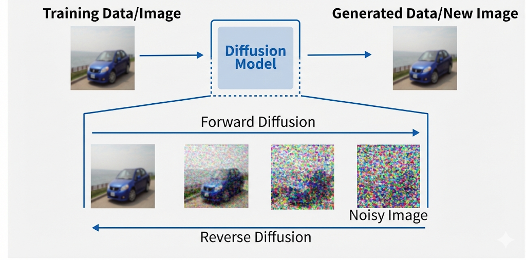
Diffusion model process

The Mathematical Foundation

Forward Process: Adding Noise

The forward process is straightforward and requires no learning. At each timestep t, a small amount of Gaussian noise is added according to a variance schedule β_t:

q(x_t | x_{t-1}) = N(x_t; √(1-β_t)x_{t-1}, β_t I)

Forward diffusion process

The key advantage of this formulation is that sampling at any timestep can be done directly using the reparameterization trick:

x_t = √(ᾱ_t)x_0 + √(1-ᾱ_t)ε

where ᾱ_t is the cumulative product of (1 — β_i) and ε ~ N(0, I).

Reverse Process: Learning to Denoise

This is where the neural network becomes essential. I train a model to predict the noise that was added, which allows me to reverse the diffusion process:

p_θ(x_{t-1} | x_t) = N(x_{t-1}; μ_θ(x_t, t), Σ_θ(x_t, t))

The mean μ_θ is computed using the predicted noise:

μ_θ(x_t, t) = (1/√α_t)(x_t - (β_t/√(1-ᾱ_t))ε_θ(x_t, t))

Implementation Details

Dataset Preparation

I used the Stanford Cars dataset (about 8000 images). The preprocessing pipeline includes:

• Resizing images to 64×64 pixels
• Random horizontal flips for data augmentation
• Normalization to [-1, 1] range
• Conversion to PyTorch tensors

U-Net Architecture

The backbone of the diffusion model is a U-Net with time conditioning. Here’s why this architecture is perfect for the task:

Symmetric Encoder-Decoder Structure: The encoder progressively downsamples the image while increasing channel depth (64 → 128 → 256 → 512 → 1024), and the decoder mirrors this process.

Skip Connections: Direct connections between encoder and decoder at matching resolutions help preserve spatial information during the denoising process.

Time Conditioning: Sinusoidal position embeddings encode the current timestep, which is crucial because the model needs to know how noisy the input is. These embeddings are projected and integrated at each resolution level.

The U-Net has a simple structure:

• Encoder: 64 → 128 → 256 → 512 → 1024 channels
• Decoder: 1024 → 512 → 256 → 128 → 64 channels
• Time embeddings injected at each level

Training Objective

Following Ho et al. (2020), I used a beautifully simple objective: predict the noise that was added.

L_simple = E_t,x_0,ε [||ε - ε_θ(x_t, t)||]

In practice, the training loop looks like this:

1. Sample a random timestep t for each image in the batch
2. Add the corresponding amount of noise to the clean image
3. Predict the noise using the U-Net
4. Compute L1 loss between actual and predicted noise
5. Backpropagate and update weights

This formulation is elegant because it’s equivalent to denoising score matching across multiple noise levels, and it’s much more stable than optimizing the full variational lower bound.

The Training Loop

for epoch in range(epochs):
    for batch in dataloader:
        # Random timestep sampling
        t = torch.randint(0, T, (BATCH_SIZE,)).long()

        # Forward diffusion
        x_noisy, noise = forward_diffusion(batch, t)

        # Predict noise
        noise_pred = model(x_noisy, t)

        # Compute loss
        loss = F.l1_loss(noise, noise_pred)

        # Optimize
        loss.backward()
        optimizer.step()

Sampling: Generating New Images

Once trained, I generated images through iterative denoising, starting from pure Gaussian noise:

Training and sampling algorithms of DDPMs. Source: Ho et al. 2020

1. Initialize: Sample x_T ~ N(0, I)
2. Iterative Denoising: For t = T down to 1:

• Predict noise using ε_θ(x_t, t)
• Compute the mean of the previous state
• Sample x_{t-1} with added stochasticity (except at t=1)

3. Output: Return the final denoised image x_0

The stochastic sampling (adding noise during generation) is key to producing diverse outputs rather than deterministic results.

Challenges and Learnings

Computational Requirements

Training diffusion models is computationally intensive. Each training step requires:

• Forward pass through the U-Net for each noisy image
• Multiple timesteps (I used T=1000)
• Sufficient batch size for stable gradients

I recommend using GPU acceleration (CUDA) and starting with smaller image resolutions (64×64) before scaling up.

Hyperparameter Tuning

The variance schedule β_t significantly impacts generation quality. I used a linear schedule from 0.0001 to 0.02, but exploring cosine schedules or learned schedules could improve results.

Training Stability

The simplified objective proved much more stable than alternatives. The L1 loss provided smoother gradients compared to L2 loss in my experiments.

Results After 100 Epochs

After training for 100 epochs, the model learned to generate recognizable car images. The progressive denoising visualization clearly shows how structure emerges from noise over the sampling steps.

Key observations:

• Early timesteps (high noise) establish rough shapes and compositions
• Middle timesteps refine object boundaries and major features
• Final timesteps add fine details and textures
• The model captures the distribution of car orientations and styles from the training data

Conclusion

100 epochs later, I have a working diffusion model that generates cars from noise. Is it perfect? No. Is it impressive compared to Stable Diffusion 3? Absolutely not. But that was never the point.

The point was understanding. And now I do.

Building this taught me more than reading ten papers. Theory gets you 60% there. Implementation gets you the other 40%. Debugging NaN gradients at 2 AM? That’s where real learning happens.

What surprised me most? The elegance. You’re just training a denoiser. That’s it. But iterate that simple idea 1000 times and you create new images from scratch. Complex behavior from simple rules.

The key takeaways:

• Diffusion models work by learning to reverse a gradual noising process
• U-Net architecture with time conditioning is essential for the denoising task
• The simplified training objective makes implementation practical and stable
• Iterative sampling allows fine-grained control over the generation process

My Implementation: https://github.com/Kaif-Imteyaz/Diffusion-Model

Resources

• DDPM (Ho et al., 2020) Start here
• Diffusion Models Beat GANs (Dhariwal & Nichol, 2021) Attention improvements
• Stanford Cars Dataset: Kaggle Dataset