The Conversation Around Tabular Data Is Back. The Tables Are Still Messy.

A hands-on walkthrough of cleaning, enriching and preparing tabular data for machine learning using skrub.

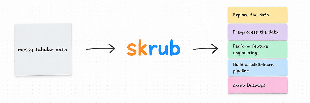
The rise of tabular foundations models (TFMs) has brought the spotlight back to tabular data. Not that it ever disappeared, I mean most businesses still run on spreadsheets and databases but the conversation around machine learning had largely shifted around other multimodal systems. However, interest in models like TabPFN and TabICL are a reminder that some of the most valuable machine learning problems are still rooted in tables.

And yet, regardless of whether you’re training gradient boosting models or experimenting with TFMs, one thing has remained unchanged which is the messy data. Data processing and cleaning remain some of the most important, and often the most time-consuming parts of any machine learning pipeline.

So how do we make working with messy tables a little less painful ? I explored some newer developments in this space and came across **skrub**, a Python library designed to make preprocessing and feature engineering easier for tabular machine learning. In this article, we’ll explore some of skrub’s features and see how they fit into a typical tabular workflow, from inspecting the data to preparing it for modeling.

This is a longer article, so feel free to treat it as a reference rather than reading it in one sitting. Companion notebooks are available in Jupyter, marimo (molab), and Kaggle if you’d like to run the examples yourself.

What is skrub?

I first came across skrub through its predecessor, [dirty_cat](https://github.com/dirty-cat/dirty_cat), which focused on one particularly frustrating aspect of working with tabular data: messy categorical values. Since then, the project has evolved into a broader toolkit for preprocessing and feature engineering on data stored in dataframes.

skrub started as dirty_cat. The project has since grown into a much broader toolkit.

At a high level, skrub sits between your dataframe and your machine learning model. It provides scikit-learn compatible tools that help with preprocessing and feature engineering while working directly with pandas and polars dataframes.

Installation & Setup

First things first, let’s start by installing skrub:

pip install skrub -U

This is enough for most of the core functionality but some features, such as TextEncoder, require some additional dependencies:

pip install skrub[transformers] -U

This will also install packages such as torch, transformers, and sentence-transformers. For this tutorial, we’ll install what we need as we go.

A Complete Workflow with skrub

Rather than looking at different features in isolation, I thought it would be more useful to see how they fit together in a typical tabular workflow.

We’ll work with a synthetic sales leads dataset where the objective is to predict whether a lead eventually converted into a customer. The target column, converted, records this observed outcome, with 1 indicating a converted lead and 0 otherwise. The dataset includes attributes such as lead source, company size, country, signup date, industry, notes, and other lead-level information.

1. Loading the data

Let’s now load the dataset and take a quick look at it. We’ll separate the target from the input features and also drop lead_id, since it simply acts as an identifier.

leads = pd.read_csv("data/messy_sales_leads.csv")

conversion_target = leads["converted"]
lead_features = leads.drop(columns=["converted", "lead_id"])
lead_features.head().T

Even the first few rows reveal several issues worth addressing before modeling.

Even from the first few rows, we can already spot several potential issues in this dataset. There are missing values, text columns that may require special handling, a column containing almost the same value throughout, and multiple representations of industry information.

2. Exploring the data

The above static preview can only tell us so much, and exploring a dataset often involves switching between multiple commands and outputs. Skrub's [TableReport](https://skrub-data.org/stable/reference/generated/skrub.TableReport.html#tablereport) combines several exploratory views into a single interactive report. Alongside summary statistics and column distributions, it also shows relationships between variables using measures such as Pearson correlation and Cramér’s V.

from skrub import TableReport
TableReport(lead_features)

TableReport generates an interactive summary of the dataset in a single line of code.

You can click on any cell in the generated table and get detailed information about the corresponding column, including missing values, the number of unique values, value distributions, and the most common categories. The dedicated Stats and Associations tabs also provide additional ways to explore the dataset, while built-in filters make it easy to focus on specific subsets of columns.

Clicking on any column reveals its distribution, null counts, and most frequent values.

If you’re working outside a notebook environment, you can also open the report directly in your browser:

TableReport(lead_features).open()

Or export it as an HTML file to share with colleagues and stakeholders:

TableReport(lead_features).write_html("lead_features_report.html")

In our dataset, we can already spot a few things that may need attention. The date columns still appear as object dtype rather than proper datetimes, and the constant_source column contains the same value for every row.

The Stats tab surfaces column-level metadata at a glance, including the constant_source column flagged for removal.

3. Pre-processing the data

Now that we have a better understanding of the dataset, it’s time to clean things up. Some issues can be fixed automatically, while others require a bit more context and standardization.

3.1 Cleaning common data issues with Cleaner

[Cleaner](https://skrub-data.org/stable/reference/generated/skrub.Cleaner.html) is a scikit-learn-compatible transformer that automates several routine preprocessing tasks, some of which are shown in the figure below.

The four routine preprocessing tasks that Cleaner handles automatically.

Let’s apply it to our dataframe and see the results.

from skrub import Cleaner
cleaned_features = Cleaner(drop_if_constant=True).fit_transform(lead_features)
cleaned_features.info()

After applying Cleaner, date columns are correctly parsed and the constant column is gone.

As we can see, the datetime columns have now been correctly parsed, and the constant_source column has been removed automatically. It is important to mention here that while Cleaner standardizes null-like values and ensures they are treated consistently across the dataframe, it does not perform imputation. Missing-value handling strategies can be applied later depending on the modeling workflow.

3.2 Joining external data with fuzzy_join

More often than not, useful data is spread across multiple tables, and bringing those tables together becomes an important preprocessing step. In our case, each lead has an office_country value but that alone doesn’t tell us much about the broader market. To add more context, we’ll bring in a small country reference dataset containing fields such as market_size_score, digital_adoption_score, average_deal_value_index, and sales_cycle_index.

countries = pd.read_csv("data/country_reference.csv")
countries.head()

The challenge however is that the country names are not written consistently. In the leads dataset, the same country may appear as USA, U.S., or United States while the reference table uses United States of America. Similarly, Brasil should match Brazil, and Espana should match Spain.

This becomes a problem because a regular pandas.merge() only works when the join keys match exactly. This is where skrub comes in handy with its [fuzzy_join()](https://skrub-data.org/stable/reference/generated/skrub.fuzzy_join.html) function which allows us to perform an approximate join instead.

from skrub import fuzzy_join
leads_enriched = fuzzy_join(
    cleaned_features,
    countries,
    left_on="office_country",
    right_on="country_name",
)

By default, fuzzy_join() matches each value to its closest counterpart in the reference table, although the matching threshold can be adjusted using the max_dist parameter.

leads_enriched[["office_country", "country_name"]].drop_duplicates().sort_values(
    "country_name"
).head(20)

fuzzy_join successfully maps messy country names like Brasil to their standardized counterparts.

3.3 Consolidating similar categories with deduplicate

The country names problem was relatively easy to solve because we had a separate reference table. But what do you do when no such table exists? In our dataset, the industry_name column contains several entries that appear to describe the same category but are written slightly differently.

sorted(cleaned_features["industry_name"].dropna().unique())

The industry_name column contains several variants of the same category, spelled slightly differently.

Should Education and Educaton be treated as different industries? What about Finanace and Finance, or Healtcare and Healthcare? In situations like these, manually cleaning categories quickly becomes tedious.

Skrub has a built-in [deduplicate()](https://skrub-data.org/stable/reference/generated/skrub.deduplicate.html#skrub.deduplicate) function for these scenarios that groups similar strings together and maps them back to a cleaner category. Under the hood, the deduplicate() function uses clustering based on string similarities to group duplicated names.

from skrub import deduplicate
cleaned_features["clean_industry_name"] = cleaned_features["industry_name"].replace(
    deduplicate(cleaned_features["industry_name"].dropna()).to_dict()
)

deduplicate() reduces 16 messy variants down to 8 clean category labels.

One thing to keep in mind is that similar-looking categories are not always the same. This step works best when spelling variations or duplicate labels genuinely refer to the same underlying category. Otherwise, important information may be lost.

From this point onward, we’ll use model_features as the dataframe passed to the modeling pipeline.

4. Performing feature engineering

After cleaning and enriching the dataset, the final step before modeling is to transform the mixed collection of numeric, categorical, datetime, and text columns into representations that machine learning models can work with. Traditionally, this would involve manually identifying column types and building separate preprocessing pipelines for each of them.

However, skrub's [TableVectorizer](https://skrub-data.org/stable/reference/generated/skrub.TableVectorizer.html) simplifies much of this process by automatically selecting suitable transformations based on the characteristics of each column.

from skrub import TableVectorizer 
vectorizer = TableVectorizer() 
encoded_lead_features = vectorizer.fit_transform(model_features)

Under the hood, TableVectorizer first runs a Cleaner on the input dataframe, splits columns based on their datatypes and number of unique values and then encodes each column according to its characteristics. By default:

• Low-cardinality categorical columns are one-hot encoded.
• High-cardinality categorical columns are transformed using StringEncoder.
• Numeric columns are passed through unchanged.
• Datetime columns are encoded using DatetimeEncoder.

A high-level view of how TableVectorizer

TableVectorizer is not a black box as the fitted vectorizer object itself is fully inspectable.

vectorizer

The fitted TableVectorizer exposes the transformers selected for each column type, along with their parameters, making the preprocessing pipeline easier to understand and debug.

You can also check how skrub classified each input column:

vectorizer.column_to_kind_

You can also check how skrub classified each input column.

The defaults are great but they are not fixed. For example, free-form text columns such as inquiry_text may benefit from richer representations using [TextEncoder](https://skrub-data.org/stable/reference/generated/skrub.TextEncoder.html#skrub.TextEncoder), which relies on pretrained language models to generate embeddings. Similarly, skrub exposes specialized transformers for handling dates, strings, and numerical features when you need more control over the preprocessing pipeline. For this walkthrough, however, we’ll stick with the defaults provided by TableVectorizer.

5. Building a predictive pipeline

The final step in our workflow is to train a predictive model. Up to this point, we’ve used TableVectorizer on its own to understand how it transforms our dataframe and to inspect the generated features. In practice, however, it is often used directly inside a scikit-learn pipeline alongside the estimator. Because TableVectorizer follows the scikit-learn API, it can be combined with virtually any scikit-learn model using the usual pipeline utilities:

from sklearn.pipeline import make_pipeline
from sklearn.ensemble import HistGradientBoostingClassifier
from skrub import TableVectorizer

pipeline = make_pipeline(
    TableVectorizer(),
    HistGradientBoostingClassifier(random_state=42),
)

TableVectorizer slots directly into a scikit-learn pipeline alongside any estimator.

Here, the dataframe first passes through TableVectorizer, which handles the feature engineering, before the resulting numerical features are used to train the classifier. But skrub also provides [tabular_pipeline](https://skrub-data.org/stable/reference/generated/skrub.tabular_pipeline.html), a convenience function that automatically combines tabular preprocessing with a scikit-learn estimator.

from skrub import tabular_pipeline 
pipeline = tabular_pipeline("classification")

If you prefer using a specific estimator, you can pass that instead.

from sklearn.linear_model import LogisticRegression 
pipeline = tabular_pipeline(LogisticRegression())

But what is happening under the hood? Well, tabular_pipeline combines the same pieces we’ve already seen:

• Depending on the estimator, it chooses an appropriate TableVectorizer configuration,
• Then, adds a SimpleImputer when missing values need explicit handling,
• Uses [SquashingScaler](https://skrub-data.org/stable/reference/generated/skrub.SquashingScaler.html) for models that benefit from scaling while skipping it for tree-based models.

As mentioned above, tabular_pipeline() adapts its defaults to the chosen estimator, as illustrated in the figure below. The [HistGradientBoostingClassifier](https://scikit-learn.org/stable/modules/generated/sklearn.ensemble.HistGradientBoostingClassifier.html) baseline relies on a simpler preprocessing workflow, while the LogisticRegression pipeline introduces additional steps such as SimpleImputer and SquashingScaler.

tabular_pipeline() adapts its defaults to the chosen estimator. The HistGradientBoostingClassifier baseline (above) uses a simpler preprocessing setup, while LogisticRegression introduces additional steps like SimpleImputer and SquashingScaler (below)

This should give a good first baseline model to start with but also gives us the flexibility to easily customize the pipeline later if needed. Once we’re happy with the setup, we can fit the pipeline and generate predictions just like we would with any other scikit-learn estimator:

pipeline.fit(model_features, conversion_target)

predictions = pipeline.predict(model_features)

conversion_probabilities = pipeline.predict_proba(
    model_features
)

Conclusion

In one of his articles, *Data Science Is Not AI, but It Is Its Genesis and Its New Frontier*, Gaël Varoquaux writes:

“AI is about automation at scale. Data science is about reasoning carefully from your data, which is more likely than not messy, biased, incomplete, and never quite what you need.”

Anyone who has worked with tabular data knows exactly why that matters. Messy data is not necessarily bad and, in many ways, reflects the complexity of the real world. The challenge, however, is learning how to work with that complexity without getting buried in repetitive preprocessing tasks. Skrub helps bridge that gap by reducing much of the boilerplate involved in preparing tabular data, making it easier to build strong baselines while still leaving room to customize the workflow when needed.