When VaR Models Break: A Regime-Based Backtesting Study Across Four Market Crises

Introduction

Value-at-Risk (VaR) is the dominant risk metric under Basel II and III. Yet every major crisis since the 1990s exposed the same pattern: models that looked adequate in calm markets failed when they were needed most.

This article asks: which VaR model breaks, and when?

Using SPY daily returns from 2005 to 2026, I backtest three models (Parametric, HS, and FHS) across ten market regimes. The results show that each model’s failure mode is predictable and regime-specific, and provide empirical support for Basel’s shift from VaR to Expected Shortfall under FRTB.

Methodology

Three VaR Models

Parametric VaR

• Assumes returns follow a normal distribution
• VaR = -(μ + z₀.₀₁ × σ), where z₀.₀₁ = -2.3263
• μ, σ estimated from rolling 250-day window
• Limitation: ignores fat tails, slow to react to volatility spikes

Historical Simulation (HS)

• No distributional assumption; uses actual past return distribution
• VaR = -(1st percentile of past 250-day returns)
• Limitation: equal-weights all 250 days, slow to reflect current volatility regime

Filtered Historical Simulation (FHS)

• Combines HS with GARCH(1,1): σ²t = ω + α × r²(t-1) + β × σ²_(t-1)
• Standardized residuals: z_t = r_t / σ_t
• VaR = -(σ_(t+1) × z₀.₀₁)
• Advantage: rapid response to volatility spikes, captures fat tails without parametric assumptions

Basel Backtesting Framework

• Rolling window: 250 trading days, consistent with the standard Basel backtesting window
• Confidence level: 99%, 1-day holding period
• Exception: actual loss exceeds VaR forecast
• Traffic Light:
• 🟢 Green: 0–4 exceptions / multiplier k = 3.0
• 🟡 Yellow: 5–9 exceptions / k = 3.4–3.8
• 🔴 Red: 10+ exceptions / k = 4.0, model review required
• Kupiec POF Test: tests whether exception rate equals theoretical 1%
• Christoffersen Test: tests time independence of exceptions (clustering detection)

Expected Shortfall (FRTB)

• FRTB replaces VaR with 97.5% ES
• ES = E[Loss | Loss > VaR]
• VaR gives only the loss threshold; ES measures average loss beyond that threshold
• Satisfies subadditivity, ensuring consistent portfolio diversification benefits

The chart below plots daily SPY returns against each model’s VaR forecast from 2005 to 2026. Each subplot represents one model. Black dots mark exceptions: days where actual loss exceeded the VaR estimate.

Three patterns are immediately visible.

• Parametric VaR remains relatively flat through GFC and COVID, systematically underestimating tail risk.
• HS adjusts more conservatively but slowly.
• FHS tracks volatility most dynamically: the line drops sharply during crisis periods and recovers gradually.

The concentration of black dots in 2008 and 2020 across all three models sets up the regime-by-regime analysis that follows.

Regime Analysis

GFC 2008: Parametric Failure

The 2008 crisis was a direct indictment of the normality assumption. Pre-GFC volatility (2006–2007) was historically low, with VIX averaging 12–15. Rolling 250-day σ estimates were suppressed, producing VaR forecasts around -1.6% per day.

• Actual losses: -8.79% (Sep 29), -9.03% (Oct 15) — 5x the model forecast
• SPY return distribution showed kurtosis of 15.38 vs normal distribution’s 3.0
• Parametric exceptions in GFC: 19 (Red Zone)
• The model was not just wrong — it was structurally incapable of capturing tail risk under a fat-tailed distribution

HS performed better (11 exceptions, Red) but still failed. Both models shared the same core problem: σ estimated from a calm period cannot capture a crisis regime.

Low-Vol Bull 2013–2019: The Hidden Volatility Problem

This regime is commonly described as a period of sustained low volatility. The data tells a more complicated story. Parametric recorded 47 exceptions (Red Zone) — the highest of any regime.

The reason is not model failure in the traditional sense. The 2013–2019 period contained five distinct volatility episodes:

• 2015 Aug: China yuan devaluation shock, SPY -4.11% in a single day
• 2016 Jan/Jun: Oil collapse + Brexit
• 2018 Feb: Volmageddon, VIX spiked from 17 to 37 overnight
• 2018 Oct–Dec: US-China trade war escalation + Fed tightening
• 2019 Aug: Tariff escalation resumption

The single-regime label “Low-Vol Bull” masked at least five mini-regimes within it. Models calibrated to the full 2013–2019 window systematically underestimated volatility during each of these episodes. This has a direct implication for risk management: regime labels are approximations, and models must be recalibrated more frequently than annual review cycles allow.

COVID 2020: FHS Adaptation Speed

COVID-19 is the cleanest demonstration of why GARCH matters. SPY fell 34% in 33 days (Feb 19 to Mar 23, 2020), the fastest drawdown of that magnitude in market history.

• Parametric: 14 exceptions (Red Zone) — rolling σ too slow to update
• HS: 8 exceptions (Yellow Zone) — flat VaR line through entire crash period
• FHS: 3 exceptions (Green Zone) — GARCH σ updated daily as volatility exploded

The mechanism is visible in Figure 3. HS VaR remained flat at approximately -6% through March and beyond, anchored by the prior 250-day window. FHS VaR spiked to -25% at the peak of the crash, tracking the actual loss distribution in near real-time.

This is the core advantage of GARCH: α × r²_(t-1) immediately incorporates yesterday’s shock into today’s variance forecast. With α ≈ 0.09 and β ≈ 0.90, volatility escalates rapidly during a crisis and decays gradually during recovery — matching the empirical behavior of financial markets.

The chart below zooms into 2020 across all three models. Each subplot covers the same date range, allowing direct comparison of how quickly each model’s VaR line responded to the crash.

The difference is structural.

• HS VaR remained flat at approximately -6% through March and beyond, anchored to the prior 250-day window.
• FHS VaR spiked to nearly -25% at the peak of the crash, with GARCH σ updating daily as volatility exploded.
• The exception count tells the same story: Parametric 14 (Red), HS 8 (Yellow), FHS 3 (Green).

2022 Bear: Correlation Breakdown

2022 was structurally different from every other regime in this analysis. The problem was not volatility estimation — it was the collapse of the stock-bond correlation that had held for 40 years.

• 1980–2021 average SPY/TLT correlation: ρ ≈ -0.3
• 2022 realized correlation: ρ ≈ +0.6
• Parametric and HS recorded Red Zone in 2022. FHS was the only exception, recording 2 exceptions (Green) — but this reflects volatility adaptation, not correlation risk management. The portfolio-level risk was still systematically underestimated.

When the Fed began its most aggressive tightening cycle since the 1980s, both equities and bonds sold off simultaneously. Single-asset VaR models are blind to this. A model estimating SPY VaR in isolation assumes nothing about what TLT is doing. In a portfolio context, this means diversification benefits were overstated and true portfolio risk was systematically underestimated throughout 2022.

This is a structural limitation that GARCH cannot fix. No amount of volatility re-estimation resolves a correlation regime shift. The solution requires multivariate modeling — at minimum, a dynamic conditional correlation (DCC) model or a t-copula framework.

The chart below plots the 60-day rolling correlation between SPY and TLT from 2005 to 2026. The 2022 period is highlighted to show the structural shift in the stock-bond relationship.

For most of the period,

• SPY and TLT moved in opposite directions: negative correlation dominated, meaning bonds provided a natural hedge against equity drawdowns.
• In 2022, that relationship broke. Correlation shifted from -0.3 to +0.6 as the Fed’s aggressive tightening cycle drove both assets down simultaneously.
• Single-asset VaR models had no mechanism to detect this. Parametric and HS entered Red Zone. FHS recorded Green Zone on exception count, but the underlying portfolio risk was equally blind to the correlation shift.

Backtesting Results

Exception Summary

The chart below summarizes exception counts by regime across all three models. The horizontal lines mark Basel Traffic Light thresholds: Green (0–4), Yellow (5–9), and Red (10+). The dashed line shows the theoretical 1% exception rate each model should produce under a well-specified model.

• Parametric exceeds the Red Zone in nearly every regime, peaking at 47 exceptions in Low-Vol Bull.
• FHS is the only model to reach Green Zone in COVID (3) and 2022 Bear (2).
• No model stays consistently near the theoretical 1% line.

Table 1 below breaks down the full exception count and Basel zone classification by regime.

Three findings stand out:

• FHS performed best in fast volatility regime shifts, recording Green Zone in COVID (3 exceptions) and 2022 Bear (2 exceptions) where adaptation speed mattered most
• No model achieves Green Zone in Low-Vol Bull — confirming that the single-regime label masked structural volatility episodes
• All three models fail over the full period — total exceptions far exceed the theoretical 51.3, and all three are rejected by statistical tests

• Parametric exception rate: 2.87% — nearly 3x the theoretical 1%, Kupiec LR = 120.07, decisively rejected
• HS and FHS exception rates closer to 1%, but both still statistically rejected
• Christoffersen test rejects independence for all three models — exceptions cluster during crisis periods, violating a core Basel assumption
• FHS Christoffersen p-value: 0.035 — closest to the 0.05 threshold, confirming GARCH partially resolves clustering but does not eliminate it

The chart below tracks the rolling Kupiec p-value for each model over the full period. Each point represents the statistical test result using the prior 250-day exception window. The red shaded areas mark periods where p < 0.05: the model is actively failing Basel’s coverage requirement.

• Parametric spends the majority of the post-GFC period below the threshold, with only brief recoveries during low-volatility windows.
• HS shows a similar but less severe pattern.
• FHS failure periods are shorter and more localized to crisis onset, with faster recovery.

No model maintains statistical validity continuously, confirming that periodic recalibration is not optional under any regime.

ES vs VaR

• ES consistently exceeds VaR across all regimes, by definition
• The gap widens most during GFC and COVID — precisely when tail losses were largest
• In 2008, average ES was approximately 1.4x the corresponding VaR estimate
• This gap represents the information VaR discards: the severity of losses beyond the threshold
• FRTB’s ES requirement directly targets this gap — forcing capital buffers to reflect not just the frequency of tail events but their magnitude

The charts below measure exceedance severity: on exception days, how large was the gap between actual loss and VaR forecast? The left panel shows average exceedance by regime. The right panel plots every exception over the full period, with average ES_975 as a reference line.

• COVID produced the largest average exceedance: Parametric (2.25%) and HS (2.2%) both exceeded 2% on exception days
• FHS recorded the lowest exceedance at 1.6%, consistent with its lower exception count of 3
• GFC: HS (1.4%) exceeded Parametric (1.25%) in severity despite fewer exceptions — when HS was wrong, it was wrong by more
• Extreme exceedances on the right panel cluster in 2008 and 2020, both well above the ES reference line
• This is precisely the information VaR discards: not whether the threshold was breached, but by how much

Implications for Risk Management

When to Recalibrate

• Yellow Zone (5–9 exceptions): re-estimate parameters. Refit GARCH α, β, consider shortening rolling window
• Red Zone (10+ exceptions): replace model or apply stressed VaR (sVaR) in parallel. Directly tied to Basel 2.5 requirements
• Exception clustering detected (Christoffersen rejected): not a parameter problem — signals regime transition. Reassess model structure
• Correlation regime shift: single-asset VaR cannot respond. Portfolio-level redesign required

Model Hierarchy by Regime

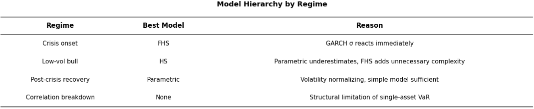
No single model dominates across all regimes. This is the core conclusion of the analysis.

FRTB Connection

• Basel II: 99% VaR, 10-day holding period
• Basel 2.5: sVaR added — mandatory separate VaR calculation using stressed period data
• FRTB : market risk capital standard moved from 99% VaR toward 97.5% ES

This transition is not regulatory convenience. The data in this analysis explains why.

• VaR only tells you the tail exists. When SPY lost -9% in a single day in 2008, a 99% VaR of -1.6% provided zero information for capital buffer sizing
• ES measures the size of the tail. Over the same period, ES tracked actual loss magnitude far more closely
• Subadditivity: VaR cannot consistently reflect portfolio diversification benefits. ES guarantees this property mathematically

Conclusion

FHS outperformed Parametric and HS across most regimes. GARCH’s daily volatility update gave it a structural advantage at crisis onset — most clearly in COVID 2020, where FHS recorded 3 exceptions (Green) against Parametric’s 14 (Red) and HS’s 8 (Yellow).

But three findings limit that claim:

• No model achieved Green Zone in Low-Vol Bull (2013–2019). Five distinct volatility episodes were hidden inside a regime labeled “low volatility”
• All three models were statistically rejected by Kupiec and Christoffersen tests. Exception clustering during crises violates the independence assumption Basel backtesting requires
• 2022 exposed the limits of single-asset VaR. FHS recorded only 2 exceptions on volatility grounds, but no model had a mechanism to detect the correlation regime shift driving the actual portfolio loss

These failures are predictable from each model’s assumptions — not random. Basel’s shift from VaR to ES under FRTB directly targets the remaining gap: tail severity, not just frequency. The logical next step is a DCC-GARCH or t-copula framework at the portfolio level, where joint tail dependency modeling would address the correlation breakdown that single-asset VaR cannot resolve.

The full code and data used in this analysis are available below.

Code: https://github.com/HoyeonJoeKang/risk-research/tree/main/var-backtesting

Data: returns.csv: https://drive.google.com/file/d/1eV7x44xjemlLgehepqdCV4fykt5OShKi/view?usp=sharing prices.csv: https://drive.google.com/file/d/1qIeyyq64bHiw-krjcmY0QIaYTgdEQpd6/view?usp=sharing