Parser Instructions: World’s fastest and most flexible protocol parsing!

This post does not reflect the views of current, past or future employers. The opinions in this article are my own. Material in this article is covered by US patent 12,461,885 “Parser instructions for CPUs”.

Protocol parsing is one of my favorite topics. I’ve talked about the basics of parsing, mechanics of parsing, and programming parsers. At the same time CPU-in-the-datapath is a lot of fun and core to my mission to prove that ultra flexibility and high performance in datapath processing are simultaneously achievable. If we combine parsing and CPU-in-the-datapath then parser instructions are the inevitable outcome. That’s the topic du jour!

At 30,000 feet, the concept of parser instructions is straightforward. It’s about creating domain specific instructions in an ISA (Instruction Set Architecture) specifically to optimize parser processing. It’s another set of instructions designed for a particular purpose sort of like how vector instructions were designed. Parser instructions provide big performance improvements by optimizing parsing in the same way that vector instructions optimize vector arithmetic operations.

As for the claim of “World’s fastest and most flexible” — I’ll put parser instructions up against any other configurable or programmable hardware solution. Parser instructions are implemented in backend hardware logic so they’re super fast, and they’re eminently flexible since they’re part of the CPU which is as programmable as anything can be. There’s also a whole bunch of advantages in making them CPU instructions in terms of leveraging existing tool chains, development practices, and operations.

Design

The design of parser instructions starts with parser design. If you recall from our previous discussions, parsing is really about processing a parse graph. A parse walk is the processing of one parse node after another for each of the constituent protocol headers in a packet. The processing for one parse node can be represented in a flow chart like:

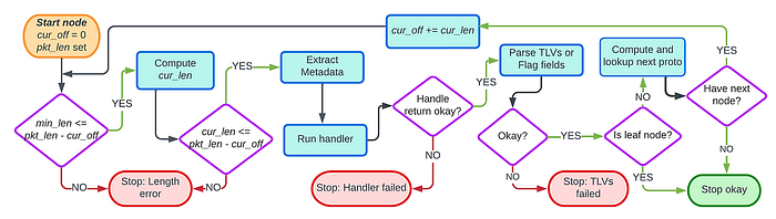
Parser instructions are used to implement the various blocks in the flow chart. Previously, we mentioned there are two critical sub-tasks in parsing: 1) Determining the length of the current header being parsed, and 2) Determining the next protocol type to parse.

On the left of the flow chart is the logic for dealing with the header length, this logic maps to a class of header length instructions. On the right is the processing to determine the type of the next protocol header and proceed to process it, this logic maps to instructions for protocol lookups and transitioning to the next parse node. Other instructions handle the functionality in the middle of the flow chart including metadata extraction, scheduling handler threads, and processing sub-nodes like TLVs.

Implementation

Parser instructions have two components: parser registers and parser instructions themselves.

Parser registers

Parser instructions include their own specialized registers called parser registers. Parser registers contain parser specific values and data and are used as input and output operands of parser instructions.

One of the most important concepts in parser instructions is the concept of a “current header” or “cursor”. As parsing proceeds, various nodes in the parse graph are processed per the headers in the packet. At any given time the CPU is processing the “current header” which is described by its offset in the packet and its header length. The current offset is in the variable cur_off of the flow chart and cur_len is the current header length. Both the current offset and length are kept in similarly named parser registers.

There’s also parser registers to hold information about the packet being processed including its length and a reference to the packet in memory. The packet length register is equivalent to pkt_len in the flow chart.

Parser instructions

We can partition parser instructions into a number of classes.

• Move instructions. Move values between integer and parser registers
• Load from header. Load 8, 16, 32, or 64 bytes from the offset of the current header into a parser register. Check the load offsets against the current header length and packet length
• Store to metadata. Store data in a register to the metadata buffer
• Length instructions. Set and check current header length
• Compare instructions. Perform logical compares of values and trap to handlers or exit the parser when a comparison fails
• CAM and array lookup instructions. A specialized CAM or array is used to perform protocol lookups and can be used for other purposes as well
• Loop instructions. Instructions that allow loops in parser processing
• Runthread. Instructions to schedule a worker thread to perform deeper processing on a protocol layer

Parser instructions are CPU instructions. This means that they can freely be intermixed with plain integer instructions or other instruction sets. This is important! It means that parser instructions are guaranteed to be part of a Turing complete instruction set. For the vast majority of protocols parsing can be done without the need to fallback to integer instructions, but for a few more complex protocols, like parsing nested protobufs, being able to intermix parser and integer instructions is a real life saver.

Instruction format

As CPU instructions, parser instructions are defined with a proper format for the ISA. Each instruction gets its own opcode number and should follow the instruction format conventions of the ISA. Our first instantiation of parser instructions is in RISC-V. We use thirty-bit instructions and custom opcodes (custom0 to *custom3* in RISC-V).

Format of RISC-V parser instructions examples. This shows the thirty-two bit RISC-V instruction formats of load, store, and length instructions

Example code

As an example of parser instructions in action, below is the assembly for parsing Ethernet and IPv4. For now, we’re just focusing on parsing itself and not worrying about processing metadata or deeper processing.

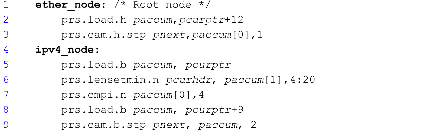
Let’s do a line item breakdown of the assembly.

Line 1: ether_node

This is a label for the Ethernet node. Presumably, ether_node is the root node of the parser. When the parser starts for a packet, parser registers are initialized and then a jump is made to the first instruction of the root node.

Line 2: prs.load.h paccum,pcurptr+12

The first instruction of ether_node is a parser load instruction. Let’s break it down:

• prs is the parser instruction prefix
• load is the opcode to load data from a source address of packet data into a parser register
• h indicates a half-word, 16 bits, is being loaded
• paccum is the destination register for the load, this is a general purpose “accumulator” parser register
• pcurptr+12 is the source for the load, this indicates that we’re loading from the address in the pcurptr register plus twelve

So what does this instruction actually do? It loads the EtherType from the Ethernet header into the accumulator register. pcurptr holds a pointer to the current header being processed, so when processing ether_node the pcurptr register points to the first byte of the Ethernet header. The source address for the load is pcurptr+12 since the offset of the EtherType field in the Ethernet header is twelve.

Line 3: prs.cam.h.stp pnext,paccum[0],1

The second instruction in ether_node is a CAM lookup instruction. This performs a lookup in a protocol table on the loaded EtherType in paccum. Let’s break it down:

• prs is the parser instruction prefix
• cam is the opcode to perform a lookup in a CAM table
• h indicates the lookup key is a half-word (16 bits)
• stp indicates end-of-node. We talk about this below
• pnext is the destination register for the result of the lookup.
• paccum[0] indicates that the input key is taken from the first half-word of the accumulator register
• 1 this is the CAM sub-table number for the lookup

This instruction performs a CAM table lookup on a key which is the low order sixteen bits of the accumulator holding the loaded EtherType. The sub-table is configured with entries for EtherType lookup, and the CAM table could be created from a protocol table in the XDP2 parser. The result of the lookup is set in the pnext register that holds the address of the next node to process.

In our example, CAM sub-table #1 includes an entry with key value of 0x800 and target value that is the address of ipv4_node. If the input packet is IPv4 then EtherType is 0x800 and the result of the lookup is that the address of ipv4_node is set in pnext register.

End-of-node processing

The last instruction executed in a node kicks off “end-of-node processing”. This is where execution jumps to the next node to process, or if parsing is complete then the parser exits and returns to the caller.

In line 3, once the CAM lookup is complete and pnext is set then the instruction performs end-of-node processing as indicated by .stp qualifier. Processing continues based on the value of the pnext register. If pnext is set to a valid address, like the address of ipv4_node in our example, then execution jumps to the address via setting the Program Counter or PC. Before the jump, pcurptr is updated to point to the next header to be processed by adding the current header length to the value in pcurptr. For Ethernet, fourteen is added to pcurptr to account for the length of the Ethernet header. But wait second, where is this being done in the code?

Setting the current header length (for Ethernet)

The pcurhdr register holds the length of the current header being parsed. When a protocol is parsed the pcurhdr register is set to reflect the length of the header. In some cases the length is set by explicit instructions as we’ll see below, but for others it’s implicit like in our example for Ethernet.

What’s the trick for setting the length of the Ethernet header? It’s the load instruction to get the EtherType. The parser load instruction does more than just load the bytes, it also deals with lengths. Firstly, the load checks that the source is within the bounds of the packet by checking that the last byte offset loaded is less than the length of the packet. If the load is for data beyond the end of the packet then the parser exits on an error.

If the load check against packet length in a load instruction succeeds then the offset of the last byte is checked against the current header length. If the loaded offset is greater than the current length then the current length is set to the last loaded offset plus one. So in the case of Ethernet, when the load of the EtherType succeeded the last offset of the load is thirteen so at that point we can set the current length register to fourteen which happens to be the length of the Ethernet header. Pretty nifty trick, huh!

Line 4: ipv4_node

This is the label for the IPv4 node. This indicates the jump point to process an IPv4 header. pcurptr is set to point to the first byte of the IPv4 header.

Line 5: prs.load.b paccum,pcurptr

The load instruction in line 5 loads the first byte of the IPv4 header that contains the IP version number and header length.

Line 6: prs.lensetmin.n pcurhdr, paccum[1],4:20

At line 6 we have an example instruction to explicitly set the current header length of a variable length header. Let’s break ‘er down:

• prs is the parser instruction prefix
• lensetmin opcode indicates we’re setting the length of a header and the min part means that we’re enforcing a minimum length
• n indicates that we’re setting the length from a nibble
• pcurhdr indicates that the length of the current header is being set
• paccum[1] indicates the input length field which is the second nibble in the paccum field (the IP header length field)
• :4 is a multiplier of the length field. The second nibble of the IPv4 header is multiplied by four to get the real length
• :20 gives the minimum header length (i.e. twenty is the minimum length of an IPv4 header)

So this instruction computes the variable length of the IPv4 header. It also checks that the header length is at least twenty bytes and the computed length doesn’t exceed the length of the packet. If any of the length checks fail then the parser exits on an error.

Line 7: prs.cmpi.n.fail paccum,4

This is a parser compare instruction to check that the IP version number is four. While the EtherType said the packet was IPv4 (i.e. it’s 0x800), we still need to check the IP version for correctness. The first nibble in the accumulator is compared to four. If the comparison is true then execution continues with the next instruction, else the parser exits on error.

Line 8: prs.load.b paccum,pcurptr+9

Load the IP protocol of the IPv4 header into the paccum register.

Line 9: prs.cam.b.stp paccum[0],2

This instruction does a CAM lookup on the IP protocol number loaded in paccum. The sub-table number is 2 and it would contain entries for TCP (key=6), UDP (key=17), etc. This is also an end-of-node instruction as indicated by the .stp prefix so either a jump is made to process the next protocol or the parser exits if the CAM lookup doesn’t return a next node.

Performance

Parser instructions are about performance. The performance comes from internal parallelism, instructions performing multiple functions, accessing multiple parser registers in an instruction with side effects, and the use of CAMs and other hardware techniques. We can compare performance of parser instructions to integer instructions by looking at the number of instructions required and the Instructions Per Cycle (IPC) each exhibits in parsing.

Each parser instruction replaces five to three hundred integer instructions with equivalent functionality. For parsing Internet protocols, we expect the ratio of parser instructions to equivalent integer instructions to be about 15:1. Parser instructions have a lower IPC that is about 0.4 on average compared to an IPC of 1.4 for parsing using integer instructions (measured on x86). Putting this together, the relative throughput speedup from parser instructions to integer instructions is 4.3. With additional optimizations to the pipeline, we expect the IPC for parser instructions will be closer to 1.0 which will further improve the speedup

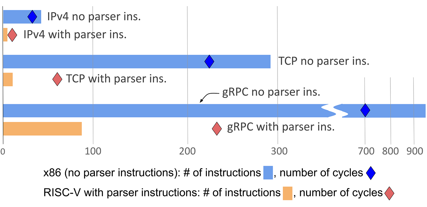
Parser instructions performance. This compares parsing using x86 integer instructions (in blue) versus RISC-V with parser instructions (in orange) to parse IPv4, TCP, and gRPC with protobufs. The solid bars give the number of instructions needed, the diamonds give the performance as the number of cycles (less is better). Note for RISC-V the number of cycles is greater than the number of instructions which implies the IPC is less than one, but for x86 the number of cycles is less than the number of instructions since the IPC is greater than one (the benefits of super scalar). The goal is to continue to increase the IPC of parser instructions