Data Structures and Algorithms Deep‑Dive — Hash Functions and Their Properties (Chapter 3, Episode 1)

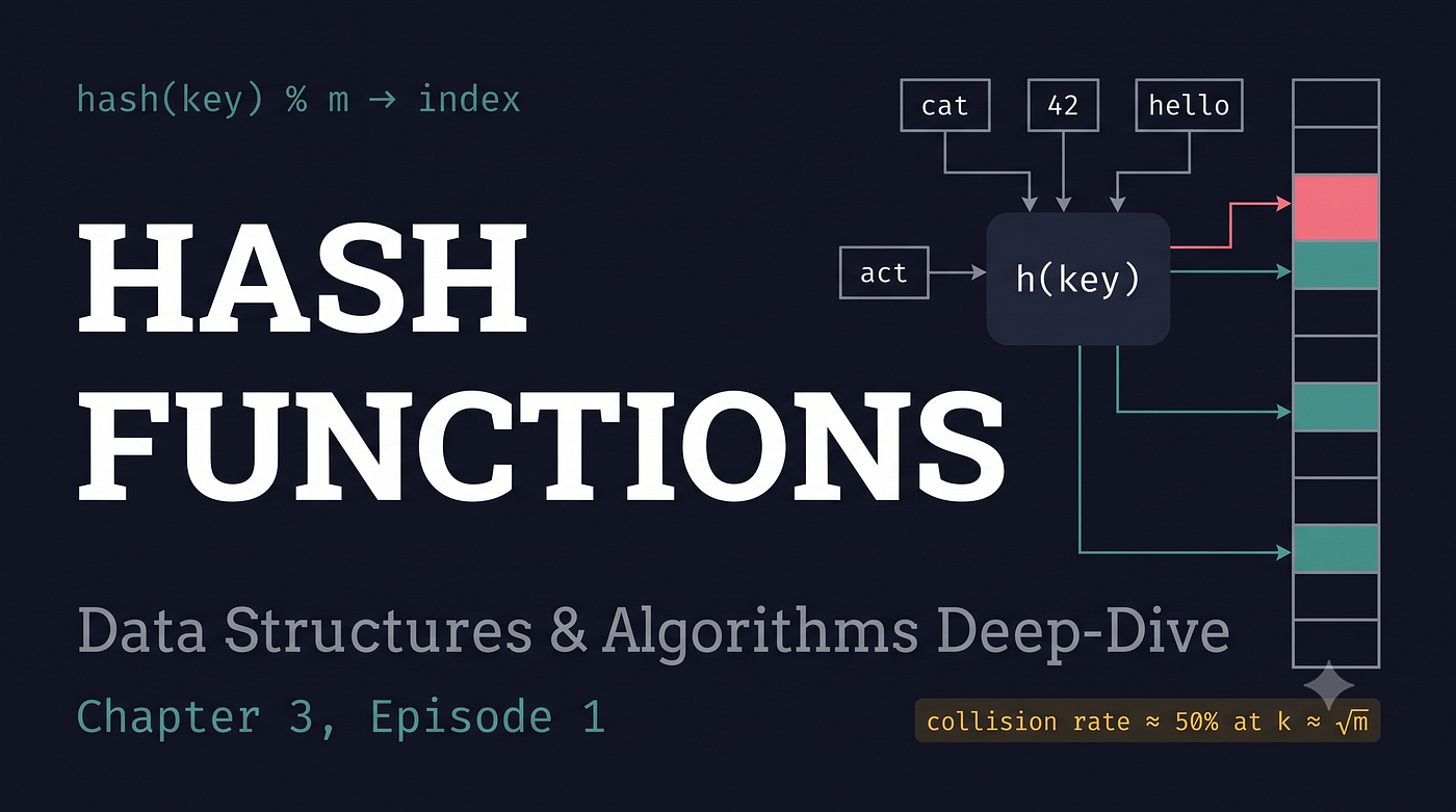
Chapter 3 — Hash Tables and Hashing

Episode 1: Hash Functions and Their Properties

Let me start this episode with a question.

You have a dictionary with a million words. Someone hands you a word and asks: “Is this word in the dictionary?” How do you find out?

If the dictionary is sorted, binary search gets you there in about 20 comparisons. That is genuinely fast. But what if I told you we could do it in — on average — one operation? Not 20. Not log n. One.

That is what a hash table does. And the mechanism behind it is completely different from anything we have built in the last two chapters. Arrays found things by position. Linked lists found things by traversal. Hash tables find things by computing where they should be.

This episode is about how that computation works — the hash function — and what makes one hash function good and another one a disaster.

Episode goals:

• Understand the core idea: mapping keys to array indices via a function
• Know what makes a hash function good: uniformity, determinism, speed, and avalanche
• Understand integer hashing, string hashing, and polynomial rolling hash
• Understand universal hashing and why it matters for adversarial inputs
• Build intuition for collision probability using the birthday bound from Episode 5

1) The Core Idea

A hash table is, at its heart, an array. When you want to store a key-value pair, instead of appending to the end, you compute the index:

index = hash(key) % table_size

hash(key) is some function that takes your key and produces an integer. The modulo operation maps that integer into the valid index range [0, table_size - 1].

To look up a key, you compute the same index and go directly there. No scanning. No comparisons on the way. Just arithmetic, then one memory access.

This is the entire idea. The sophistication — and all the interesting problems — live in two places: designing a good hash function, and handling the case where two different keys compute to the same index (a collision). This episode covers the first. Episode 2 covers the second.

2) What Makes a Hash Function Good?

Before we look at specific hash functions, it helps to know what we are aiming for. A good hash function has four properties.

Deterministic. The same key must always produce the same index. This sounds obvious, but it rules out hash functions that use random numbers, current timestamps, or any non-reproducible state. If hash("apple") returns 42 on insert and 17 on lookup, you will never find anything.

Uniform distribution. Keys should spread as evenly as possible across the table. If all keys cluster at indices 0–10 regardless of table size, you effectively have a 10-slot table, not a 1000-slot one. The collision rate goes up, performance degrades, and the theoretical O(1) average case becomes O(n) in practice.

Fast to compute. A hash function that takes O(n) time per key lookup defeats the purpose. Ideally, hashing a key takes O(1) or O(key length) time — fast enough that it does not dominate the overall operation cost.

Avalanche effect. A small change in the key should produce a large, unpredictable change in the hash value. If hash("cat") and hash("bat") differ by only one bit, keys that are similar in value will cluster together in the table. Good hash functions amplify small input differences into large output differences.

3) Hashing Integers

The simplest case: your key is an integer k, and your table has size m.

Division method:

hash(k) = k % m

Simple and fast. But the choice of m matters enormously.

If m is a power of 2 (say, m = 2^p), then k % m just takes the last p bits of k. If your keys have patterns in their low bits (which is common — think even-numbered IDs, aligned memory addresses), many keys will map to the same bucket. The hash becomes as bad as the pattern in the data.

Rule of thumb: choose m to be a prime not close to a power of 2. For example, if you want a table of roughly 1000 slots, use m = 997. The prime ensures that the structure of m does not interact with patterns in the keys.

Multiplication method:

hash(k) = ⌊m × (k × A mod 1)⌋

where A is a constant with 0 < A < 1. Knuth suggests A ≈ (√5–1)/2 ≈ 0.618 (the inverse golden ratio).

The idea: multiply k by A, take the fractional part, then scale to [0, m). The multiplication mixes the bits of k, and the golden ratio constant has good distribution properties across a wide range of input patterns. The table size m can be a power of 2 here — the multiplication does the mixing, so m’s structure does not matter.

4) Hashing Strings

Strings are the most common key type in practice. How do you hash a variable-length sequence of characters into a single integer?

Naive approach — sum of character codes:

hash("cat") = ord('c') + ord('a') + ord('t') = 99 + 97 + 116 = 312

This is fast but terrible. “cat”, “act”, and “tac” all hash to 312. Any permutation of the same characters produces the same hash. For natural language dictionaries, where anagrams are common, this causes massive clustering.

Polynomial rolling hash:

Treat the string as a polynomial in a base b, evaluated at that base, modulo a prime p:

hash(s) = (s[0] × b^(n-1) + s[1] × b^(n-2) + ... + s[n-1] × b^0) mod p

In code:

hash(s):
  h ← 0
  for each character c in s:
    h ← (h × b + ord(c)) mod p
  return h

Each character is mixed into the accumulator via multiplication by base b before adding the next character. Position matters — “cat” and “act” now produce different hashes because character positions affect the result differently.

Typical values: b = 31 or 37 (small primes), p = 10⁹ + 7 or 10⁹ + 9 (large primes). The large prime prevents overflow from dominating and keeps the hash in a manageable range.

Why this works well: the polynomial structure ensures that every character contributes to the final value in a position-dependent way. The prime modulus distributes values across the range. The multiplication by base b is the “mixing” step — it prevents the additive cancellation that broke the naive sum approach.

5) The Rabin-Karp Rolling Hash

Polynomial hashing has a beautiful extension for substring search: the rolling hash. Instead of recomputing the hash of each new substring from scratch (O(n) per window), you update it in O(1) by adding one character and removing another.

For a window of length k:

hash(s[i+1..i+k]) = (hash(s[i..i+k-1]) × b - s[i] × b^k + s[i+k]) mod p

Slide the window right: multiply the current hash by b (shifts all existing characters one position left), subtract the contribution of the character leaving the window, add the new character.

This is O(1) per slide, O(n) total for an n-character string with window k. The naive approach would be O(nk). We will use this in Chapter 10 (String Algorithms) for the Rabin-Karp pattern matching algorithm. I am introducing the hash mechanics now because they belong here.

6) Collision Probability — The Birthday Bound Revisited

From Episode 5 of Chapter 1: if you insert k keys into a table of size m, the probability of at least one collision is approximately:

1 - e^(-k(k-1) / 2m)

This exceeds 50% when k ≈ √(2m ln 2) ≈ 1.17√m.

For a table of size m = 10⁶, collisions become likely after only k ≈ 1170 insertions. That is 0.1% of the table capacity.

This is the birthday bound, and it has a practical implication that surprises many engineers: a hash table starts having meaningful collision rates long before it is full. This is exactly why load factor management (covering in Episode 3) matters — you rarely want to fill a hash table beyond 70–75% capacity.

For the hash function to delay collisions as long as possible, it needs to distribute keys truly uniformly. A biased hash function that favours certain indices will hit collisions far earlier than the birthday bound predicts — essentially, the effective table size is smaller than m.

7) Non-Cryptographic vs Cryptographic Hash Functions

Not all hash functions are made for hash tables. It is worth knowing the distinction.

Non-cryptographic hash functions (MurmurHash, xxHash, FNV, CityHash): designed for speed and good distribution. Suitable for hash tables. Not suitable for security — an adversary who knows the hash function can craft inputs that all collide, turning your O(1) hash table into an O(n) linked list and crashing your server. This is a real class of denial-of-service attack.

Cryptographic hash functions (SHA-256, SHA-3, BLAKE3): designed to be computationally infeasible to reverse or to find collisions deliberately. Much slower (tens of bytes per nanosecond vs hundreds). Used in digital signatures, password storage, and data integrity checks. Overkill for hash tables.

Most language runtimes use non-cryptographic hash functions with a randomly-chosen secret seed per process run. Python uses SipHash-1–3 (a keyed, fast hash) for string and bytes keys. The secret seed means an adversary cannot predict hash values across different process runs — defeating most collision-based attacks.

8) Universal Hashing

Here is a problem. Any fixed hash function h can be defeated by a sufficiently adversarial input set — there will always exist some set of keys that all hash to the same bucket. This is a mathematical certainty: with n keys and m buckets, by the pigeonhole principle, any fixed function will map some set of ⌈n/m⌉ keys to the same bucket.

Universal hashing solves this by randomising the hash function at runtime, rather than fixing it at design time.

A universal hash family H is a set of hash functions such that for any two distinct keys x ≠ y:

P_{h ∈ H}[h(x) = h(y)] ≤ 1/m

When we pick h randomly from H at table construction time, the probability of any specific pair of keys colliding is at most 1/m — regardless of what the keys are.

A simple universal family for integer keys:

h_{a,b}(k) = ((a × k + b) mod p) mod m

where p is a prime larger than the key universe, and a ∈ {1,…,p-1}, b ∈ {0,…,p-1} are chosen uniformly at random.

Why this is universal: for any x ≠ y, the probability over random (a,b) that h(x) = h(y) is exactly 1/p ≤ 1/m (since p ≥ m). The proof uses the fact that for any distinct x,y, the map (x,y) → (h(x), h(y)) is a bijection over choices of (a,b), so exactly 1/p of (a,b) choices produce a collision.

Practical implication: with universal hashing, the expected number of collisions for any input set is O(n/m) — regardless of adversarial input. This is the theoretical guarantee that makes hash tables safe.

9) What Python and Java Actually Do

It is worth grounding the theory in what real runtimes implement, since you will use these systems every day.

Python:

• Integers: hash(n) = n for small integers; modified for large ones to stay in range.
• Strings: SipHash-1–3 with a random seed chosen per process. Two runs of the same Python program hash the same string to different values (by default). This is PYTHONHASHSEED behaviour introduced in Python 3.3 as a security fix.
• Custom objects: __hash__ defaults to object identity (id(obj) // 16). If you override __eq__, you must override __hash__ — objects that compare equal must hash equally.

Java:

• String.hashCode() uses the polynomial rolling hash with b=31: s[0]*31^(n-1) + s[1]*31^(n-2) + .... This is a fixed function — the same for every JVM, which makes Java strings vulnerable to collision attacks if used in adversarial contexts without additional protection.
• HashMap uses a secondary "mixing" function on top of hashCode() to improve distribution.

The key takeaway: production hash functions are not naive. But even good hash functions can be gamed if the attacker knows the function and the seed. Understanding universal hashing tells you why randomisation matters.

10) Common Pitfalls

Using a bad hash function because “it works on examples.” A hash function that distributes well on your test data may cluster badly on production data. Test on adversarial inputs, not just random ones.

Mutable objects as hash keys. If an object’s hash changes after insertion (because the object was mutated), you will never find it again — it is now at the wrong index. Python makes strings, integers, and tuples hashable (immutable) but lists and dicts unhashable for exactly this reason.

Forgetting that equal objects must have equal hashes. This is a mathematical requirement, not a style preference. If a == b but hash(a) != hash(b), the hash table is broken — lookups will fail even when the key is present.

Choosing table size as a power of 2 with a bad hash function. As discussed in §3, a power-of-2 table with a hash function that does not adequately mix bits concentrates keys in a small subset of buckets. Use a prime table size or a mixing-heavy hash function.

Ignoring the birthday bound. Expecting a hash table to work well at 95% load is wishful thinking. At that load, the expected number of collisions is very high regardless of hash quality.

11) Practice Exercises

Level A — Direct Application:

1. Compute hash("hello") using the polynomial rolling hash with b=31, p=10^9+7. Work through character by character: 'h'=104, 'e'=101, 'l'=108, 'l'=108, 'o'=111.
2. For a hash table of size m=7 (prime), hash the integers [12, 19, 5, 26, 33, 40] using k % m. Are any collisions produced?
3. Explain why “abc” and “bca” produce the same hash under the naive sum method but different hashes under the polynomial rolling hash with b=31.

Level B — Analysis: 4. A hash table has m=100 slots. Using the birthday bound, estimate how many insertions are needed before the probability of at least one collision exceeds 50%. Compare to intuition. 5. The multiplicative hash hash(k) = ⌊m × (k × 0.618 mod 1)⌋ with m=8: compute hashes for k = 1, 2, 3, 4, 5, 6, 7, 8. Comment on the distribution compared to k % 8. 6. A web server uses hash(ip_address) % num_buckets to route requests to backend servers. An attacker sends requests from IPs that all hash to the same bucket. What is the attack and what is the fix?

Level C — Deeper Reasoning: 7. Prove that the family h_{a,b}(k) = ((ak + b) mod p) mod m is universal. Specifically, show that for any distinct x, y, the number of pairs (a,b) with h_{a,b}(x) = h_{a,b}(y) is exactly p(p-1)/m — and therefore the probability is 1/m when (a,b) is chosen uniformly at random. 8. Design a hash function for 2D integer point keys (x, y). It should not treat (x,y) and (y,x) as identical. State your base, prime, and mixing strategy, and argue why your choice avoids the anagram problem. 9. Python's PYTHONHASHSEED=0 disables hash randomisation. Write a proof-of-concept (in pseudocode) that, given a fixed non-randomised polynomial hash function with known b and p, an adversary can construct n strings that all hash to the same bucket in O(n) time.

Hints:

• For 1: h = 0; h = (0×31 + 104) % p = 104; h = (104×31 + 101) % p = 3325; continue for ‘l’, ‘l’, ‘o’.
• For 7: for distinct x,y, (ax+b) ≡ (ay+b) mod p iff a(x-y) ≡ 0 mod p iff a ≡ 0 mod p (since p is prime and x≠y mod p). But a ∈ {1,...,p-1} excludes a=0, so no pair (a,b) collides in the inner modulus. The collision in the outer mod m happens whenever (ax+b mod p) and (ay+b mod p) fall in the same block of size p/m. Count carefully.
• For 8: hash((x,y)) = (x * b + y) % p for large prime p. This treats the pair as a two-character string — positional mixing distinguishes (x,y) from (y,x) whenever x ≠ y.

12) Summary and What’s Next

Here is what this episode covered:

The hash function is the mechanism that makes O(1) average-case lookup possible — it maps a key to an array index via arithmetic rather than comparison or traversal. A good hash function is deterministic, uniformly distributing, fast, and exhibits the avalanche effect.

Integer hashing works well with prime table sizes and the division method, or with the multiplication method using the golden ratio constant. String hashing uses polynomial rolling hash — position-dependent, mixing via multiplication by base b. Universal hash families randomise the function to defeat adversarial inputs, guaranteeing expected O(1/m) collision probability for any pair of distinct keys.

The birthday bound tells us collisions become likely well before the table is full — around √m insertions for a table of size m. This is the mathematical reason load factor management matters.

Next episode (Chapter 3, Episode 2): Collision Resolution Strategies.

Now that we know how keys are mapped to indices, we need to deal with the inevitable fact that two keys will sometimes land on the same index. Episode 2 covers the two major strategies: chaining (each bucket holds a linked list of colliding keys) and open addressing (find another slot in the same array). Both have subtleties that affect performance in ways that are not obvious at first glance.

13) Further Reading

• Cormen, Leiserson, Rivest, Stein — Introduction to Algorithms (CLRS), Chapter 11 (Hash Tables) — the universal hashing proof is particularly thorough here
• Knuth — The Art of Computer Programming, Vol. 3, Section 6.4 (Hashing)
• MurmurHash, xxHash documentation — for what production non-cryptographic hash functions actually look like
• Python documentation — object.__hash__ and notes on hash randomisation

Appendix: Reference Implementations

Python — Polynomial rolling hash:

def poly_hash(s: str, base: int = 31, mod: int = 10**9 + 7) -> int:
    h = 0
    for ch in s:
        h = (h * base + ord(ch)) % mod
    return h

# Verify anagram sensitivity
print(poly_hash("cat"))  # some value
print(poly_hash("act"))  # different value — position matters
print(poly_hash("tac"))  # different again

Python — Rabin-Karp rolling hash (sliding window):

def rolling_hashes(s: str, k: int, base: int = 31, mod: int = 10**9 + 7):
    """Yield (start_index, hash) for every substring of length k."""
    if len(s) < k:
        return

    # Precompute base^k mod p
    bk = pow(base, k, mod)

    # Hash of first window
    h = 0
    for i in range(k):
        h = (h * base + ord(s[i])) % mod
    yield 0, h

    for i in range(k, len(s)):
        # Slide: add s[i], remove s[i-k]
        h = (h * base + ord(s[i]) - ord(s[i - k]) * bk) % mod
        yield i - k + 1, h

for idx, h in rolling_hashes("abcabc", 3):
    print(f"s[{idx}:{idx+3}] = {'abcabc'[idx:idx+3]!r}  hash={h}")

Python — Universal hash family for integers:

import random

class UniversalHash:
    def __init__(self, m: int, p: int = 10**9 + 7):
        self.m = m
        self.p = p
        self.a = random.randint(1, p - 1)
        self.b = random.randint(0, p - 1)

    def hash(self, k: int) -> int:
        return ((self.a * k + self.b) % self.p) % self.m

# Two instances use different (a,b) — defeats adversarial construction
h1 = UniversalHash(m=100)
h2 = UniversalHash(m=100)
keys = [42, 137, 256, 999, 1024]
print("h1:", [h1.hash(k) for k in keys])
print("h2:", [h2.hash(k) for k in keys])  # different distribution

Python — Checking the birthday bound empirically:

import random
import math

def collision_prob_empirical(m: int, k: int, trials: int = 10000) -> float:
    hits = 0
    for _ in range(trials):
        seen = set()
        for _ in range(k):
            idx = random.randrange(m)
            if idx in seen:
                hits += 1
                break
            seen.add(idx)
    return hits / trials

m = 365
for k in [10, 23, 30, 50]:
    empirical    = collision_prob_empirical(m, k)
    theoretical  = 1 - math.exp(-k*(k-1)/(2*m))
    print(f"k={k:3d}  empirical={empirical:.3f}  theoretical={theoretical:.3f}")