How do you differentiate code? Automatic Differentiation (AAD) Walkthrough

So you’re presenting your new model, painstakingly trained and optimised, to your stakeholders. It’s going well and people are impressed with the results until it becomes time for the Q&A.

“What happens if we tweak this parameter just slightly?” Your boss’s boss asks. You answer, according to the mathematical theory.

But your boss’s boss doesn’t care about theory and the what ifs keep coming. What if customer churn increased by 1%? What about a change in ad clicks? You know theoretically that this is a basic question, it’s just differentiation, easy when your model is something like linear regression. But you don’t know the derivative of pipeline.fit_transform(data).

But if you did, well that would be a gamechanger. You’d be able to calculate the sensitivity to parameters left, right and centre. There’d be significantly less panicking when it becomes time to present to stakeholders at the very least and with that new found confidence you can look great in front of your boss’ boss!

It just relies on answering one question: How on earth do you differentiate a programming language?

Differentiation using symbols

There are a number of skills that humans do well and machines don’t. One thing computers don’t tend to do as well is differentiation. Not the actual maths, it’s a deterministic set of rules of course, but being able to understand code at a mathematical level.

YOU can probably do it well because you wrote the code with an understanding of the mathematics behind it. But for a computer, looking at foo(x) and interpreting it as actual symbols to differentiate is a whole different kettle of fish. Computers execute instructions, they don’t abstractly think about them.

Now work has been done to try and overcome this limitation. Sympy for example is a library that does enable understanding of mathematics on a symbolic level and therefore allows differentiation as well. But there are a few problems with it.

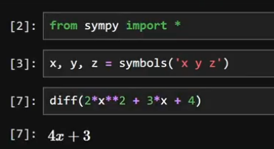
Using Sympy for symbolic differentiation

The basic functionality behind it is that you do express your code in mathematical symbols, ones that you can pass to sympy and then it can use the standard differentiation rules like the chain, product and quotient rules to do the actual differentiation.

Chain, Product and Quotient rules, created via Manim

But the problem with this is that not only do we have to write our code in a way that is computer understandable and hopefully efficient from an execution perspective, we also have to write it in a way that is Sympy understandable for the differentiation.

You can already see how easy it could be to get these two out of sync. It also doesn’t solve the underlying problem: The system still can’t reason about our code mathematically. Our code is full of complex logic: data cleaning, business logic, feature engineering. You’re never actually differentiating something like 2x² + 3x + 4, but a complicated combination of mathematical and and data munging operations.

I mean let’s go through an example of code that I wrote earlier, this code to make google trends data actually usable for machine learning. I’ve got a function f which is a function of the input trends data and its batch number.

Example code to try and convert to sympy

If I want to differentiate it with respect to a change in just one day, x_i, I have a function that is a sum over a number divided by a sum, multiplied by a sum.

(Approximate) Mathematical representation of the above code

Honestly, I’m not even sure I’ve got this mathematical representation completely correct. What makes sense in programming doesn’t always make sense to show symbolically, which makes it even harder to turn business logic into something we can differentiate.

But say we could differentiate it. We have a couple of product rules to apply but the real issue is that I’m working vectorised in this code.

Vectorising code adds an additional layer of complexity when it comes to attempting symbolic differentiation

This means I can write it in a way that’s quite simple, just a few lines, but in reality it works very differently under the hood.

Differentiating vectorised code means handling each vectorised term like it’s a massive loop. You can immediately see how the amount of symbols starts to become so big that it is frankly unmanageable.

This is called expression swell and even with a small project like my own this becomes unmanageable. Over a bigger project you’ll find your memory blowing before symbolic differentiation even has chance to finish. On top of that, if-else statements cause blowups if we happen to step over a discontinuity.

Expression swell as a relatively simple function is differentiated multiple times

It’s a nice little package that works in theory, but like much theory, the translation to the complexities of real world problems falls apart.

Now that’s not the only method we can use to differentiate something. In finance we used to do something called “bump and reprice”: Change one of the input variables just slightly and re-run the function with the new input.

This works on the basis of Taylor Expansion. The Taylor expansion of function x at point a = x + h is:

Taylor expansion formula

Which we can rearrange to get:

Rearranged Taylor expansion

Now how well this works all depends on how large this some error is. Because if h is 0.1 then h² is 0.01, h³ is 0.001 and so on, making the terms smaller and smaller. So again, in theory, a small bump means a more accurate differential.

However, small bumps have their own issue and that’s the size of a float. You can only go too close to zero before you lose precision and your float gets rounded down to zero itself. Most floats are float32. You could try making your floats have 64bit precision but then we find ourselves in a situation where memory is blowing up again. So it’s a tradeoff. Bump and reprice is a simpler calculation, but it comes with a cost in accuracy.

That’s not the only cost either. Bump and reprice is slow. Sometimes, very slow. Not only do you calculate the original function, but you run the exact same function again for the bumped and repriced version.

Bump and reprice pseudocode

Which takes twice as long if we’re bumping just one variable, but this waiting around scales with the number of sensitivities as well. If you have 1000 inputs, you’re waiting for 1000 model runs to get all the sensitivities.

Not only are we sacrificing accuracy, we’re sacrificing time as well.

The holy grail then is to be able to calculate sensitivities both accurately and efficiently and in the majority of data science those things tend to be at odds with one another. However, this is a rare case where we can make one thing that does both, enter automatic differentiation.

Now I wanted a high level explanation of automatic differentiation that I could give you here but the reason no ELI5 exists is because this isn’t easy. The way we’re going to do this is how most explanations structure it, we’re going to look at the forward method to get an understanding and then talk about the backwards method that is actually efficient and useful for automatic differentiation.

So let’s start with function f which is function that depends on input w. Now w is not the raw data, but it depends on the raw data variable c and some function v. Moving down a layer, let’s say v depends on u and some raw data a and then finally u is a function of a, b and c, which is all our raw data.

Our functions for the worked example

The question your boss’s boss raised in the opening of this video? That’s asking for df/da, df/db and df/dc. How does f change with respect to a, b and c? That’s what automatic differentiation is going to find out.

Now in order to be able to start differentiating, we need to understand the dependency graph. I just gave you it in the set up of the functions but if you can’t trace your way through the code then automatic differentiation is a non-starter.

So what I just described looks a little bit like this:

Dependency graph for our worked example

The other mathematical concept it’s important to know here is what the jacobian is. That’s a matrix of partial derivatives. So if we have a function g of variables x1,…, xn then the Jacobian of g, Jg = (dg/dx1, …, dg/dxn).

So knowing that u is a function of a, b and c, we can compute its jacobian (du/da, du/db, du/dc).

We then move up a layer. v is a function of u and a, so we can compute its jacobian, (dv/da, dv/du).

Now the chain rule states that we can calculate dv/da by dv/du * du/da and so if we put it in matrix form that looks like:

dv/da in matrix form

And we can add columns to the latter matrix to get dv/db and dv/dc as well:

Matrix to calculate dv/da, dv/db and dv/dc

Now we already have the top line from the jacobian earlier and the bottom line is trivial, da/da is 1, da/db and da/dc are both zero. So that gives us:

The Jacobian of v, expressed by matrix multipllication of derivates of lower level functions

We can continue to move up the graph.

W is a function of c and v, so the Jacobian of w is given by:

Matrix form of the Jacobian of w

So we’re literally stacking the jacobian of c underneath the jacobian of v.

Continue up a layer, evaluating all the matrix multiplications and we’ve finally got a Jacobian for f.

In order to work out the actual sensitivities to a, b and c, we only need to multiply this matrix by (1, 0, 0), (0, 1, 0) and (0, 0, 1) respectively.

We get the derivatives of f by multiplying the Jacobian of f by the respective vectors for a, b and c

Now there are two problems with what I’ve got here. Firstly is that I’ve been keeping track of the Jacobian’s symbolically, keeping it in terms of partial derivatives. In practise, storing a matrix like this would be huge from a memory perspective, a bit like the expression swell I mentioned when discussing Sympy.

Instead, forward mode AD calculates the matrix multiplications locally at each point, “on the fly” so to speak as we go through the graph.

In order to do this, we need a starting point, a seed vector to multiply by. And as we’re calculating the sensitivities, we’re better off choosing one that isolates just one variable.

For example if we wanted to get the sensitivity of f to a we could choose (1, 0, 0) as our starting point. However, this also means that we would have to rerun the same calculation with vectors (0, 1, 0) and (0, 0, 1) to get the sensitivity with respect to b and c as well.

And you may be wondering okay now we’re talking about real numbers instead of symbols. How does it actually DO the differentiation with real numbers? And the answer is simple: We can break the ultimate computation down into primitives, basic mathematical operations such as addition, multiplication, sin, etc. All of these things we know how to differentiate.

So that table of differentiation formulas you learned when you first saw calculus is effectively built-in to the system. This allows us to apply the relevant product, chain and quotient rules to calculate the full derivative.

The way this is done is often through overloaded operators. That’s basically changing how addition fundamentally works so that it returns both the value, the normal result of addition, and the tangent, the derivative propagated down to this addition. The same is true for all primitives.

But the whole reason we didn’t do bump and reprice is because we’d have to re-run the function for every single input we wanted to bump. Forward Automatic Differentiation is just doing the same thing. But here’s the beauty of it: We’re not actually going to do this forward method, we’re going to go backwards instead. And we can re-use the maths we did already for it. So instead we start at the top, calculating the sensitivities back from the output.

So what does that look like? Instead of seeding at the bottom, we start at the top.

Every variable keeps an adjoint which we write as xbar. That adjoint represents how much our output function f depends on that variable x. So xbar = df/dx. That means that as we go down, wbar will be df/dw and v bar will be df/dv. We ultimately want to calculate abar, bbar and cbar.

Note that the symbol we bar is the symbol on the bottom of the derivative, and all derivatives are of f

We have to choose somewhere to start the calculation so that it’s not symbolic and so we’ll use fbar = df/df = 1.

Then we get wbar = df/dw = df/dw 1 = df/dw fbar where we calculate wbar using our overloaded operators.

Calculating wbar

Moving down vbar = df/dv = df/dw dw/dv = wbar dw/dv which we calculate again using our overloaded operators.

Calculating vbar

As we calculate our way all the way down the dependency graph we reach the bottom where we can calculate abar, bbar and cbar via one backward sweep and have our sensitivities.

Once we’ve moved down the graph calculating abar, bbar and cbar we can get our final sensitivities in one backwards sweep.

However, there’s one important caveat here. In order to do this, we need to know two things: The path which we came from, and the previous values of fbar, xbar and wbar. This means that we need to be storing those values as we go down, as well as the values we’re calculating for f, w, v, u etc so we can use them in the calculation. This is the biggest drawback of reverse mode, the need to store these values on the way down. This is known as the tape of operations.

But what it suffers with in storage it makes up for lightning speed and accuracy. Instead of needing to bump and reprice or run through the graph for each variable, it gives us the benefit of all variables in one go, provided you store the incremental steps along the way.

So if you have an AAD implemented framework and your boss asks you what happens if you change this variable? You’ll have the answer, all given in one calculation.

Of course the devil is in the detail. Implementing AAD is very hard. While loops, conditional statements, external library calls all make AAD a nightmare. So why not impress your boss’s boss by using a platform that does it for you?

The Evil Works PUFF platform is looking for early partners to put our calculation efficiency to the test. If you’d like to help shape the development of the platform, get in touch at evilworks.com/contact.