Building Interpretable Models with ID3 Decision Trees

Photo by Jefferson Santos on Unsplash

Imagine you’re trying to explain a big decision to someone — like choosing a new phone. You might break it down into questions: “Do I want iOS or Android?” “Is the camera quality important?” “What’s my budget?” Based on the answers, you narrow down your choices until you find the perfect phone. That’s basically how a decision tree works in machine learning!

Decision trees are one of the most intuitive and interpretable machine learning models out there. Unlike complex black-box models (looking at you, deep learning), decision trees provide clear, step-by-step reasoning behind their predictions. This makes them a go-to choice when transparency is just as important as accuracy — think healthcare, finance, or legal decisions where understanding why a model made a choice is critical.

One of the earliest and most well-known decision tree algorithms is ID3 (Iterative Dichotomiser 3). It’s a foundational technique that uses a concept called information gain to build a tree that efficiently classifies data. In this article, we’ll break down how ID3 works, why it’s useful, and how you can implement it yourself. Let’s dive in! 🚀

Understanding Decision Trees

Photo by bruce mars on Unsplash

Alright, let’s break down decision trees in a way that makes sense. Imagine you’re playing 20 Questions — you start with a broad question like “Is it an animal?” and keep narrowing things down based on yes/no answers until you land on the right answer. That’s exactly how decision trees work in machine learning!

A decision tree is made up of:

• Nodes (questions we ask about the data)
• Branches (possible answers leading to more questions or a final decision)
• Leaves (final classifications or predictions)

For example, let’s say you’re trying to classify whether an email is spam or not. A decision tree might start by asking: Does the email contain the word “free”? If yes, it moves one way. If no, it moves another. It keeps splitting based on the most informative features until it reaches a conclusion: Spam or Not Spam.

Why Use Decision Trees?

✅ Super easy to interpret — Unlike neural networks, which are basically a tangled mess of numbers, decision trees lay out their reasoning in a way that humans can understand. ✅ No need for a ton of data prep — They can handle missing values and don’t require fancy scaling techniques like some other algorithms. ✅ Works well for classification — If you need a clear-cut answer (Yes/No, Cat/Dog, Fraud/Not Fraud), decision trees are a great fit.

The Downsides?

❌ They can overfit — A tree can get too specific to the training data, making it less effective on new data. ❌ Not always the most accurate — Simplicity comes at a cost, and sometimes other models (like random forests) perform better.

Despite their quirks, decision trees are a fantastic tool for building interpretable machine learning models — especially when you use smart algorithms like ID3, which we’ll dive into next! 🚀

The ID3 Algorithm Explained

Photo by ThisisEngineering on Unsplash

Now that we know how decision trees work, let’s talk about ID3 (Iterative Dichotomiser 3) — one of the OG algorithms for building them. It’s been around since the ’80s (shoutout to Ross Quinlan for inventing it), but it’s still a great way to create simple, interpretable models.

So, how does ID3 actually build a decision tree? It all comes down to entropy and information gain — two fancy terms that help us figure out which feature to split on at each step.

Step 1: Understanding Entropy (a.k.a. Messiness of Data)

Entropy is just a way of measuring how pure or messy a dataset is. If a dataset is perfectly ordered (e.g., all emails are spam), entropy is low. If it’s a mixed bag of spam and not spam, entropy is high.

Think of it like sorting socks. If all your socks are already paired up, life is good (low entropy). But if they’re all jumbled in a drawer, you’ve got a mess to deal with (high entropy).

Mathematically, entropy is calculated like this:

…where pip_ipi​ is the probability of each class in the dataset. Don’t worry too much about the math — it just helps us measure disorder.

Step 2: Information Gain (Choosing the Best Split)

Now that we know entropy tells us how messy things are, information gain tells us how much we can clean things up by splitting on a certain feature. ID3 looks at all the features and picks the one that reduces entropy the most — in other words, the best question to ask first.

Formula for information gain:

This just means:

• Take the original entropy
• Subtract the weighted entropy of splitting by a feature
• The bigger the reduction, the better the feature to split on

Step 3: Building the Tree

Once we have the best feature to split on, we:

1. Create a new node for that feature
2. Split the data into subsets based on the feature’s values
3. Repeat the process on each subset until we reach pure groups (all of one class)

Let’s say we’re classifying fruits, and our features are color, size, and shape. ID3 might find that color is the best feature to split on first. If we separate red fruits from yellow and green ones, we’ve already made a big dent in the classification problem. Then, we repeat the process for each subset!

Example Walkthrough

Imagine we have this tiny dataset:

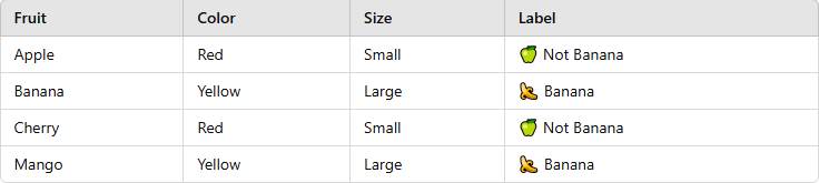
• Step 1: Calculate entropy of the dataset.
• Step 2: Check which feature (Color or Size) gives the highest information gain.
• Step 3: Split the data using the best feature.
• Step 4: Repeat until all groups are pure (all “Banana” or “Not Banana”).

Boom! You’ve got yourself a decision tree built with ID3! 🎉

ID3 is a great starting point for decision trees, but it has some limitations — like only working with categorical data. That’s why later algorithms like C4.5 and CART came along to improve on it. But if you want to understand the core ideas behind decision trees, ID3 is a solid place to start.

Next up, let’s see how we can actually code this in Python! 🐍💻

Implementing ID3 in Python

Photo by Mohammad Rahmani on Unsplash

Alright, now that we understand how ID3 works, let’s get our hands dirty and actually code it in Python! 🐍💻

Before we start, we have two options:

1. Use an existing library like scikit-learn (easy but less educational).
2. Build ID3 from scratch (more fun and helps you understand the logic).

Let’s go with option 2 and build it ourselves! 🚀

Step 1: Import Required Libraries

We don’t need much — just numpy and pandas for handling data and a bit of math.

import numpy as np
import pandas as pd
from collections import Counter

Step 2: Define Entropy Calculation

Entropy measures how messy our dataset is. Here’s a simple function to compute it:

def entropy(data):
    labels = data.iloc[:, -1]  # Last column is the target label
    label_counts = Counter(labels)
    total = len(labels)

    return -sum((count/total) * np.log2(count/total) for count in label_counts.values())

This function takes a dataset and tells us how mixed the labels are. Lower entropy = better splits!

Step 3: Compute Information Gain

Now, we’ll define a function that calculates which feature gives the best split by maximizing information gain.

def information_gain(data, feature):
    total_entropy = entropy(data)
    values = data[feature].unique()

    weighted_entropy = sum(
        (len(data[data[feature] == value]) / len(data)) * entropy(data[data[feature] == value])
        for value in values
    )

    return total_entropy - weighted_entropy

This function loops through all possible values of a feature, splits the data, and calculates the drop in entropy.

Step 4: Build the ID3 Algorithm

Now, let’s recursively build our decision tree!

def id3(data, features):
    labels = data.iloc[:, -1]

    # Base case: if all labels are the same, return that label
    if len(set(labels)) == 1:
        return labels.iloc[0]

    # Base case: if no features left, return the most common label
    if not features:
        return labels.mode()[0]

    # Find the best feature to split on
    best_feature = max(features, key=lambda f: information_gain(data, f))

    tree = {best_feature: {}}
    features = [f for f in features if f != best_feature]

    # Recursively build the tree for each value of the best feature
    for value in data[best_feature].unique():
        subset = data[data[best_feature] == value]
        tree[best_feature][value] = id3(subset, features)

    return tree

This function: ✅ Checks if all labels are the same (then we’re done). ✅ Picks the feature with the highest information gain. ✅ Recursively splits the dataset until we reach pure groups.

Step 5: Test It on a Sample Dataset

Let’s try it on a simple fruit classification problem.

# Sample dataset
data = pd.DataFrame({
    'Color': ['Red', 'Yellow', 'Red', 'Yellow'],
    'Size': ['Small', 'Large', 'Small', 'Large'],
    'Label': ['Not Banana', 'Banana', 'Not Banana', 'Banana']
})

features = list(data.columns[:-1])  # Exclude the label column

# Build the decision tree
tree = id3(data, features)
print(tree)

Expected Output (something like this):

{'Color': {'Red': 'Not Banana', 'Yellow': 'Banana'}}

Our tree learns that red fruits are not bananas, and yellow fruits are bananas. 🍌🔥

Step 6: Making Predictions

Now, let’s write a function to classify new examples using our decision tree.

def classify(tree, sample):
    if not isinstance(tree, dict):
        return tree  # Leaf node reached, return label

    feature = next(iter(tree))
    value = sample[feature]

    if value in tree[feature]:
        return classify(tree[feature][value], sample)
    else:
        return "Unknown"  # Handle unseen values

Example usage:

sample = {'Color': 'Red', 'Size': 'Small'}
print(classify(tree, sample))  # Output: "Not Banana"

Boom! 🎉 We just built an ID3 decision tree from scratch!

✅ No fancy libraries needed — just core Python ✅ Step-by-step breakdown of entropy, information gain, and recursion ✅ Clear and interpretable results

While this was a basic example, you can expand it to handle larger datasets, numerical features, and even pruning techniques to improve accuracy. But for now, pat yourself on the back — you just built your own decision tree classifier! 💪

Next up, let’s talk about evaluating and improving our model to make it even better. 🚀

Evaluating and Improving Model Performance

Photo by Danial Igdery on Unsplash

Alright, we’ve built our ID3 decision tree, but how do we know if it’s actually good? And what if it’s making mistakes? 🤔 In this section, we’ll cover ways to evaluate and improve our model so it doesn’t fall apart when faced with new data.

Step 1: Evaluating Model Accuracy

A simple way to check how well our decision tree is doing is by calculating accuracy — the percentage of correct predictions. If we have a test dataset, we can compare our model’s predictions to the actual labels.

def accuracy(tree, test_data):
    correct = sum(classify(tree, row) == row['Label'] for _, row in test_data.iterrows())
    return correct / len(test_data) * 100

Then, we can test it with some new data:

test_data = pd.DataFrame({
    'Color': ['Yellow', 'Red', 'Yellow', 'Red'],
    'Size': ['Large', 'Small', 'Small', 'Large'],
    'Label': ['Banana', 'Not Banana', 'Banana', 'Not Banana']
})

print(f"Model Accuracy: {accuracy(tree, test_data)}%")

If we get 100% accuracy, great! But real-world datasets are messy, so let’s talk about common problems and how to fix them.

Step 2: Handling Overfitting

Overfitting happens when our tree memorizes the training data too well and struggles with new examples. It’s like learning every single question on a practice test but failing when the real exam has different questions. 😅

How to Fix It:

✅ Pruning (Trimming the Tree) — Cut off unnecessary branches to make the tree simpler. ✅ Setting a Maximum Depth — Stop the tree from growing too deep and capturing noise. ✅ Using More Data — A larger dataset helps the tree generalize better.

Let’s implement pruning by limiting how deep the tree can grow:

def id3_with_depth(data, features, depth=0, max_depth=3):
    labels = data.iloc[:, -1]

    if len(set(labels)) == 1:
        return labels.iloc[0]

    if not features or depth == max_depth:
        return labels.mode()[0]  # Return the most common label

    best_feature = max(features, key=lambda f: information_gain(data, f))
    tree = {best_feature: {}}
    features = [f for f in features if f != best_feature]

    for value in data[best_feature].unique():
        subset = data[data[best_feature] == value]
        tree[best_feature][value] = id3_with_depth(subset, features, depth + 1, max_depth)

    return tree

Now, we can control how deep the tree goes, reducing overfitting! 🎯

Step 3: Comparing ID3 with Other Decision Tree Algorithms

ID3 is great, but it has some limitations, like only working with categorical data (no numbers). That’s why more advanced versions exist:

If you want a better-performing tree, try using scikit-learn’s built-in DecisionTreeClassifier:

from sklearn.tree import DecisionTreeClassifier

clf = DecisionTreeClassifier(criterion='entropy', max_depth=3)
clf.fit(train_data.drop(columns=['Label']), train_data['Label'])
predictions = clf.predict(test_data.drop(columns=['Label']))

This saves a ton of time compared to writing ID3 from scratch!

Step 4: Preprocessing Data for Better Results

A good model starts with clean, well-prepared data. Here’s how you can make sure your decision tree gets the best input:

✅ Convert categorical data to numbers (if using a library that requires it) ✅ Handle missing values (fill them with the most common value) ✅ Remove unnecessary features (irrelevant data can confuse the tree)

For example, if our dataset has missing values, we can fill them like this:

data.fillna(data.mode().iloc[0], inplace=True)

This makes sure our tree doesn’t break due to missing info.

Great, now you know how to evaluate and improve your decision tree! 🌟

✔️ We checked model accuracy ✔️ We tackled overfitting with pruning ✔️ We compared ID3 with better algorithms ✔️ We learned how to clean data for better performance

Up next, let’s explore real-world applications of ID3 — where this algorithm actually shines! 🚀

Real-World Applications of ID3 Decision Trees

Photo by bruce mars on Unsplash

Alright, we’ve built our ID3 decision tree, improved it, and even tested it. But you might be wondering: Where is this actually used in the real world? 🤔 Well, ID3 (and decision trees in general) are super useful in various industries where clear, interpretable decisions matter. Let’s check out some cool real-world applications! 🚀

1. Spam Email Detection 📧

Ever wonder how your email provider knows which emails to send straight to the spam folder? Decision trees help! An ID3-based model might classify emails based on features like:

✅ Does it contain “free money” or “win now”? ✅ Is the sender unknown? ✅ Does it have lots of exclamation marks (!!!)?

By analyzing past emails, the tree can learn patterns and automatically flag new spam messages before they even hit your inbox. Say goodbye to sketchy “You’ve won a free iPhone!” emails. 🎉

2. Medical Diagnosis 🏥

Doctors use decision trees to help diagnose diseases based on symptoms. Let’s say a patient comes in with:

🤒 Fever? → Yes 🤧 Cough? → Yes 😷 Shortness of breath? → No

A decision tree might classify this as a common cold instead of something more serious like pneumonia. ID3 can help doctors make quick, data-driven decisions while keeping the process transparent for patients.

3. Credit Scoring & Loan Approvals 💰

Banks don’t just hand out loans to anyone (unfortunately 😅). They use decision trees to decide who’s likely to pay back a loan and who isn’t. Some key factors they look at:

✅ Credit score (high or low?) ✅ Employment status (stable job or unemployed?) ✅ Debt-to-income ratio (can they afford to pay it back?)

The ID3 algorithm helps banks quickly assess risk and make fair, consistent decisions without human bias.

4. Customer Churn Prediction 📉

Businesses want to keep their customers happy, so they use decision trees to predict who might leave (churn) and why. They analyze factors like:

✅ How often does the customer use the product? ✅ Have they contacted customer support recently? ✅ Did they downgrade their subscription?

By identifying at-risk customers early, companies can offer discounts or better support to keep them around. It’s like Netflix knowing exactly when to send you that “Hey, come back for a free month!” email. 🎥

5. Fraud Detection 🔍

Credit card fraud is a big problem, and decision trees help catch suspicious transactions in real-time. If a bank sees:

❌ Large purchase in another country? ❌ Happened at 3 AM? ❌ Customer has never shopped there before?

The model might flag the transaction for review before money is lost. Pretty smart, right?

6. Recommendation Systems 🎵🎬

Ever wonder how Spotify or Netflix seem to know exactly what you want to watch or listen to? Decision trees play a role in personalized recommendations! They analyze things like:

✅ What genres do you like? ✅ Do you prefer action movies or rom-coms? ✅ Have you skipped similar songs before?

The model then suggests content tailored to you — like how YouTube keeps recommending videos even when you promised yourself “just one more.” 😆

As you can see, decision trees (and ID3 in particular) aren’t just an academic exercise — they power real-world applications that affect us daily. Whether it’s detecting spam, approving loans, diagnosing diseases, or stopping fraud, decision trees help make data-driven decisions easy to understand.

So next time you get a “Suspicious login attempt” email or a perfectly curated Netflix recommendation, just remember — there’s probably a decision tree working behind the scenes! 🌳🔍

Now that we’ve covered everything, let’s wrap this up with some final thoughts and next steps! 🚀

Conclusion and Next Steps

Wow, we’ve covered a lot! 🎉 From understanding how ID3 decision trees work to implementing them in Python and exploring their real-world applications, you’ve taken a deep dive into one of the most interpretable machine learning algorithms out there.

So, let’s do a quick recap:

✅ ID3 Basics — It’s a rule-based, interpretable decision tree algorithm that uses entropy and information gain to split data. ✅ Implementation — We built ID3 from scratch in Python (because we’re awesome like that 😎). ✅ Evaluating and Improving — We learned about overfitting, pruning, and accuracy to make our model better. ✅ Real-World Uses — ID3 isn’t just theory; it’s used for spam detection, fraud prevention, medical diagnoses, and more!

But what’s next? 🤔

Where to Go From Here?

If you’re excited to keep learning, here are some ideas for your next steps:

🔥 Try More Advanced Decision Trees — Check out C4.5, CART, or Random Forests to see how they improve on ID3. 📊 Work with Bigger Datasets — Test your ID3 model on real-world datasets like those from Kaggle or UCI Machine Learning Repository. 🔧 Use Scikit-Learn — If you want a more optimized approach, try sklearn.tree.DecisionTreeClassifier to see how pros do it. 🚀 Apply it to a Real Problem – Have a dataset? Build a decision tree model to classify customers, predict outcomes, or detect patterns.

Final Thoughts

ID3 decision trees might be one of the simplest machine learning algorithms, but they’re also powerful and easy to interpret — making them a great starting point for any ML journey. Whether you’re building models for fun, school, or work, decision trees are a fantastic tool to have in your AI toolbox.

So, what’s your next project? Will you test ID3 on a new dataset? Or maybe dive into more advanced algorithms? Whatever you choose, keep experimenting, keep coding, and most importantly — have fun with it! 🚀💡

And if you ever need help? You know where to find me. 😉