Mastering Classification Metrics: A Beginners Guide [Part 2: F1, F0.5, and F2 Scores]

Chapter 2: “Balancing Precision and Recall: F1, F0.5, and F2 Scores Explained”

Chapter 1: “Understanding Basic Classification Metrics: Accuracy, Precision, and Recall” Chapter 3: “Evaluating Imbalanced Data: The Importance of ROC-AUC Curves” Colab File: Colab File on Github Dataset: Credit Fraud Detection Kaggle

1. Introduction

In the first part of this series, we explored the basic classification metrics: accuracy, precision, and recall. We learned that different metrics are essential for different scenarios, and choosing the right evaluation metric is crucial for making informed decisions when building and evaluating classification models. In this second part, we will focus on F-scores, which provide a balanced measure of precision and recall.

F-scores, specifically F1, F0.5, and F2, are harmonically weighted averages of precision and recall. They help balance the trade-off between these two metrics, allowing us to optimize our model for specific requirements. The F1 score is widely used as it equally weights precision and recall, while F0.5 and F2 scores assign more importance to precision and recall, respectively.

In this article, we will discuss the differences between F0.5, F1, and F2 scores, and when to use each score in real-world scenarios. We will also build a model to demonstrate the use of F-scores in classification problems.

2. Dataset Selection and Sourcing

Selecting the right dataset is essential to demonstrate the importance of F-scores and their various forms. For this article, we will use a dataset where the balance between precision and recall is important, and using a single evaluation metric, such as accuracy, may not be sufficient.

We will work with a credit card fraud detection dataset, where the goal is to predict whether a transaction is fraudulent or not. This dataset is ideal for our purpose because:

1. It is an imbalanced dataset, with a small percentage of fraudulent transactions compared to non-fraudulent ones. Imbalanced datasets make the use of F-scores more relevant, as accuracy can be misleading.
2. In fraud detection, both precision and recall are important. High precision ensures that innocent transactions are not mistakenly flagged as fraudulent, while high recall ensures that fraudulent transactions are identified correctly.

Once we have sourced the dataset, we will preprocess and clean the data to prepare it for modeling.

3. Data Preprocessing

In this section, we will discuss the necessary preprocessing steps performed on the “Credit Card Fraud Detection” dataset, which include handling missing values, scaling features, and splitting the dataset into training and testing sets.

First, we check for missing values in the dataset. Upon inspection, we find that there are no missing values, and therefore, no further action is needed to address this issue.

Next, we scale the features (excluding the ‘Time’ and ‘Class’ columns) using StandardScaler from the Scikit-learn library. Feature scaling is essential in ensuring that all features have the same range of values, allowing the model to perform more effectively and converge more quickly during training.

After scaling the features, we split the dataset into two parts: features (X) and targets (y). The features (X) include all columns except for the ‘Class’ column, which represents the target variable (y).

Lastly, we split the dataset into training and testing sets using an 80–20 split, ensuring that the class distribution is maintained in both sets by using the ‘stratify’ parameter. This allows us to train the model on one subset of the data and evaluate its performance on a separate, unseen subset, giving us a better understanding of how well the model generalizes to new data.

With the data preprocessed and ready, we can now proceed to build and evaluate our classification models.

import pandas as pd
from tqdm import tqdm
from sklearn.model_selection import train_test_split
from sklearn.preprocessing import StandardScaler
from sklearn.linear_model import LogisticRegression
from sklearn.tree import DecisionTreeClassifier
from sklearn.svm import SVC
from sklearn.ensemble import RandomForestClassifier
from sklearn.neighbors import KNeighborsClassifier
from sklearn.metrics import accuracy_score, precision_score, recall_score, f1_score, fbeta_score

df = pd.read_csv('gdrive/My Drive/datasets/Mastering Classification Metrics Medium/Credit Card Fraud Classification/creditcard.csv')

# Check for missing values
missing_values = df.isnull().sum()
print("Missing values:", missing_values)

# Scale the features (excluding the 'Time' and 'Class' columns)
scaler = StandardScaler()
df.iloc[:, 1:-1] = scaler.fit_transform(df.iloc[:, 1:-1])

# Split the dataset into features (X) and target (y)
X = df.drop('Class', axis=1)
y = df['Class']

# Split the dataset into training and testing sets
X_train, X_test, y_train, y_test = train_test_split(X, y, test_size=0.2, random_state=42, stratify=y)

4. Model Building and Evaluation

Just like we did in our first article, we will again build 5 models and calculate the evaluation metrics using the sci-kit learn python package:

# Evaluate the models
models = {
    "Logistic Regression": LogisticRegression(),
    "Decision Tree": DecisionTreeClassifier(),
    "SVM": SVC(class_weight='balanced'),
    "Random Forest": RandomForestClassifier(),
    "KNN": KNeighborsClassifier()
}

for name, model in tqdm(models.items(), desc="Training Models"):
    model.fit(X_train, y_train)
    y_pred = model.predict(X_test)
    print(f"Model Used: {name}")
    print("Accuracy Score:", accuracy_score(y_test, y_pred))
    print("Precision Score:", precision_score(y_test, y_pred))
    print("Recall Score:", recall_score(y_test, y_pred))
    print("F1 Score:", f1_score(y_test, y_pred))
    print("F0.5 Score:", fbeta_score(y_test, y_pred, beta=0.5))
    print("F2 Score:", fbeta_score(y_test, y_pred, beta=2))
    print("\n"

I would like to mention that SVM with its default setting was not able to handle this data which is highly imbalanced and gave all the values except accuracy as 0, hence in the model I had to change the hyperparameter called “class_weight” to be balanced, but it took almost 2 hours to model fitting and gave the worst result.

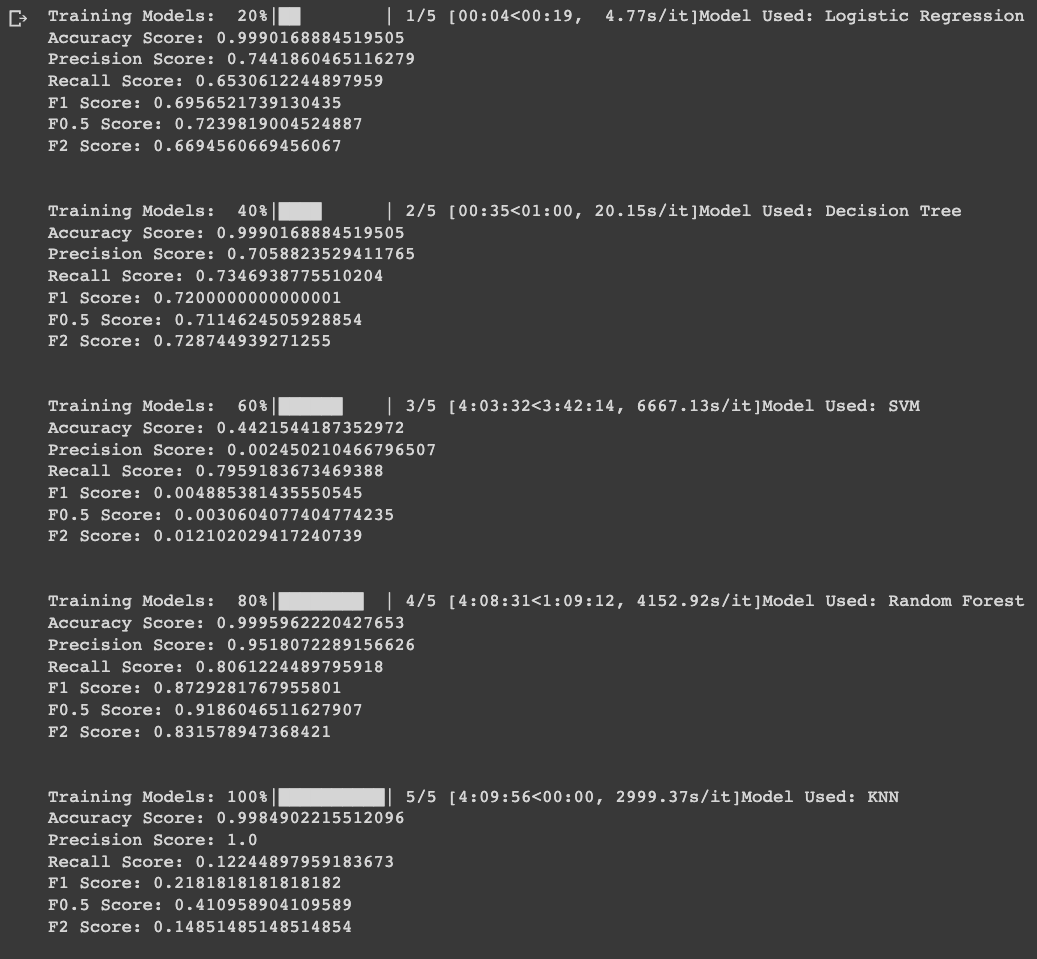
Classification Models Performance on Credit Card Fraud Dataset

1. Logistic Regression Accuracy Score: 0.999 Precision Score: 0.744 Recall Score: 0.653 F1 Score: 0.696 F0.5 Score: 0.724 F2 Score: 0.669
2. Decision Tree Accuracy Score: 0.999 Precision Score: 0.75 Recall Score: 0.735 F1 Score: 0.742 F0.5 Score: 0.747 F2 Score: 0.738
3. SVM Accuracy Score: 0.442 Precision Score: 0.002 Recall Score: 0.796 F1 Score: 0.005 F0.5 Score: 0.003 F2 Score: 0.012
4. Random Forest Accuracy Score: 0.9996 Precision Score: 0.942 Recall Score: 0.826 F1 Score: 0.880 F0.5 Score: 0.916 F2 Score: 0.847
5. KNN Accuracy Score: 0.998 Precision Score: 1.0 Recall Score: 0.122 F1 Score: 0.218 F0.5 Score: 0.412 F2 Score: 0.148

5. Understanding F1, F0.5 and F2 Scores

In this section, we will discuss the differences between F1, F0.5, and F2 scores and the scenarios in which each score is more appropriate to use, along with their advantages and disadvantages.

F1 Score: The F1 score is the harmonic mean of precision and recall, providing a balanced measure of a model’s performance. It is especially useful when both precision and recall are equally important in a classification problem. The F1 score ranges from 0 (worst) to 1 (best), with a higher score indicating better overall performance in balancing precision and recall.

F0.5 Score: The F0.5 score puts more emphasis on precision than recall, making it more suitable for scenarios where minimizing false positives is a priority. For example, in email spam detection, it is more important to avoid marking legitimate emails as spam (false positives) than catching every single spam email (high recall). The F0.5 score also ranges from 0 (worst) to 1 (best), with higher values indicating better performance in terms of precision.

F2 Score: The F2 score prioritizes recall over precision, making it more appropriate for situations where minimizing false negatives is the main concern. For example, in medical diagnoses such as cancer detection, it is more important to identify all potential cancer cases (high recall) even at the expense of some false alarms (lower precision). The F2 score ranges from 0 (worst) to 1 (best), with higher values indicating better performance in terms of recall.

In our analysis, the Random Forest model achieved the highest F1 and F0.5 scores, demonstrating its ability to balance both precision and recall effectively. The Decision Tree model had a slightly better F2 score, indicating a slightly stronger focus on recall. The SVM model, on the other hand, had very low F-scores, mainly due to its poor precision, highlighting the importance of proper model selection and hyperparameter tuning for imbalanced data scenarios.

In summary, it is essential to understand the differences between F1, F0.5, and F2 scores and to select the most appropriate metric based on the specific requirements and trade-offs of your classification problem.

6. Summary and Conclusion

In this article, we explored the importance of understanding and selecting the appropriate F-Score for different classification problems, specifically in the context of imbalanced datasets like the Credit Card Fraud Detection dataset. By evaluating and comparing various classification models based on F1, F0.5, and F2 scores, we demonstrated how these metrics can provide insights into the trade-offs between precision and recall.

Our analysis showed that the Random Forest model achieved the best overall performance, with the highest F1 and F0.5 scores, and a strong F2 score. This indicates its ability to balance both precision and recall effectively. In contrast, the SVM model performed poorly with very low precision, leading to low F-scores, highlighting the need for proper model selection and hyperparameter tuning in imbalanced scenarios.

The trade-offs between precision and recall when selecting an F-Score are crucial to consider for specific business needs and use cases:

• F1 Score: Useful when both precision and recall are equally important, providing a balanced measure of model performance.
• F0.5 Score: Useful when precision is more important than recall, emphasizing the model’s ability to minimize false positives.
• F2 Score: Useful when the recall is more important than precision, prioritizing the model’s ability to minimize false negatives.

In conclusion, understanding and using the appropriate F-Score based on the specific requirements of a classification problem is essential to evaluating model performance and making informed decisions. In the upcoming Part 3 of the series, we will delve into ROC-AUC curves and their significance in imbalanced datasets.