Complete Guide to Linear Algebra Using Python- Part 1- Vectors— The Building Blocks of Data
Introduction: Bridging the Gap
Complete Guide to Linear Algebra Using Python- Part 1- Vectors— The Building Blocks of Data
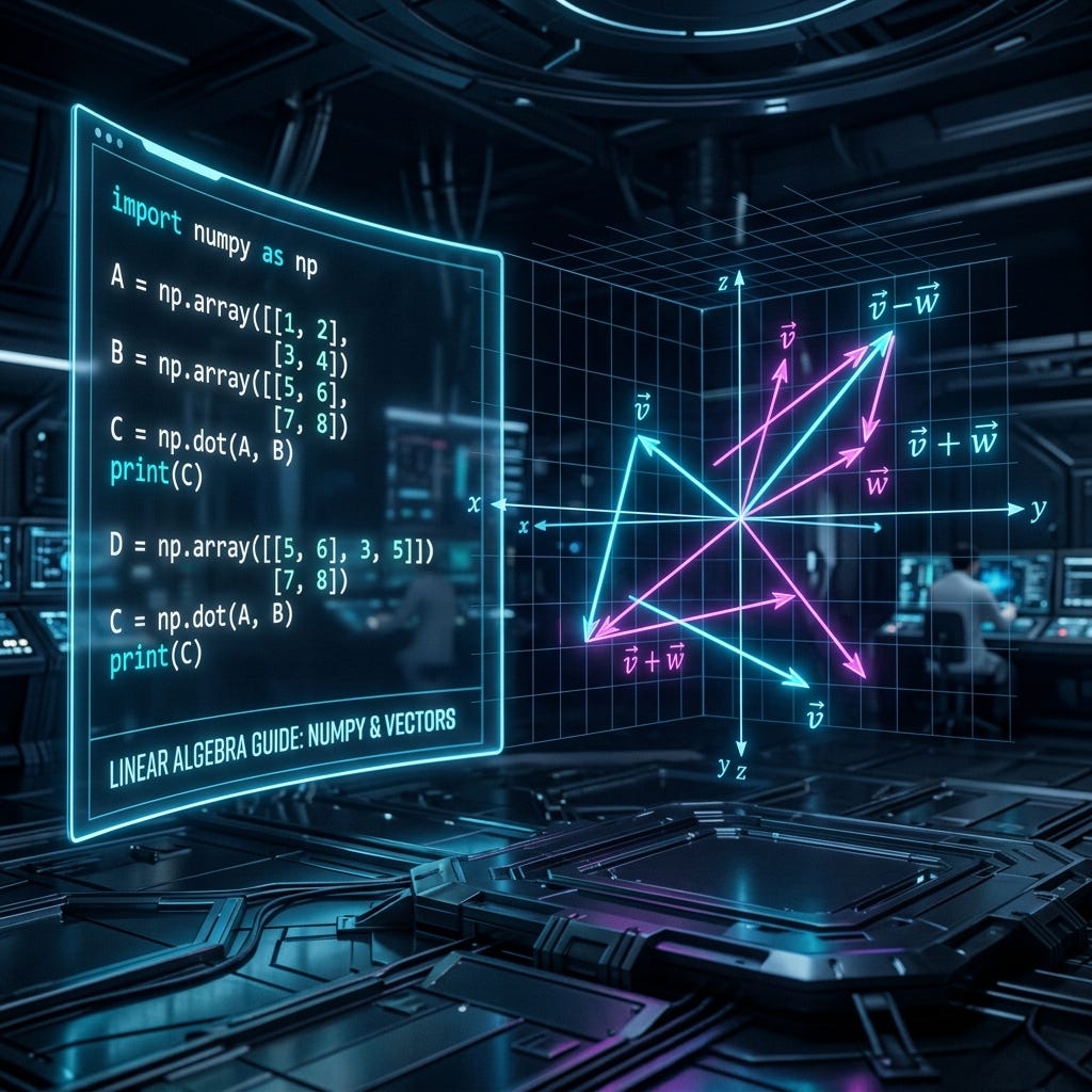
Introduction: Bridging the Gap
If you have a background in Economics, Statistics, or Mathematics, you are likely familiar with the theoretical elegance of Linear Algebra. Textbooks like Introduction to Linear Algebra by Gilbert Strang are fantastic for teaching the proofs and the pencil-and-paper mechanics. However, in research and industry, we rarely solve these problems by hand.
The challenge for many academics is the “implementation gap” — knowing the theorem but not knowing how to translate it into a computational tool. This series is designed to bridge that gap. We will take the rigorous structure of classic Linear Algebra and implement it using Python, specifically the NumPy and SymPy libraries.
Our goal is to move from abstract n-tuples to working code that can power simulations, regressions, and data models.
0. The Toolkit: Setting Up Your Linear Algebra Lab
Before we dive into the math, we need the right tools. Linear algebra in the 21st century is best explored through code.
The IDE: VS Code & Jupyter Notebooks For this series, I highly recommend using Visual Studio Code (VS Code) with the Jupyter Extension.
- Why? It allows you to run code cells individually, seeing your matrices and plots immediately after you write them.
Installation Open your terminal or command prompt and run the following command to install the essential libraries:
pip install numpy sympy pandas matplotlib
Importing the Libraries At the top of your notebook, start by importing these powerhouse packages:
import numpy as np # Numerical computing (The workhorse)
import sympy as sp # Symbolic math (For textbook-style solutions)
import pandas as pd # Data manipulation
import matplotlib.pyplot as plt # Visualizations
I highly recommend that you copy the codes and run it yourself to see how they work.
1. What is a Vector? In its simplest form, a vector is just a list of numbers. In physics, it’s often described as something with magnitude and direction. In Linear Algebra, we view it as a point in space or an n-tuple of numbers.
The Notation: In math textbooks, you’ll see vectors represented as u = (u₁, u₂, …, uₙ). In Python, we use NumPy arrays.
# Defining a 3 dimensional vector u = [1, 2, 3]
u = np.array([1, 2, 3])
print(f”Vector u: {u}”)
2. The Two Core Operations Almost everything in linear algebra is built on two simple operations:
A. Vector Addition To add two vectors, they must have the same dimension. You simply add the corresponding components. Mathematical Rule: u + v = (u₁ + v₁, u₂ + v₂, …, uₙ + vₙ)
# Vector Addition
u = np.array([1, 2, 3])
v = np.array([4, 5, 6])
sum_uv = u + v
print(f"u + v = {sum_uv}") # Output: [5, 7, 9]
B. Scalar Multiplication A scalar is just a single number (like 3 or -0.5). When you multiply a vector by a scalar, you multiply every component of the vector by that number. Mathematical Rule: ku = (ku₁, k u₂, …, k uₙ)
# Scalar Multiplication
k = 3
u=np.array([1,2,3])
scaled_u = k * u
print(f"3 * u = {scaled_u}") # Output: [3, 6, 9]
Linear Combinations
A linear combination is simply the result of adding scaled vectors together. If we have vectors u and v and scalars a and b, the linear combination is w = au + bv.
In Python, this is incredibly straightforward:
a, b = 2, -1
u = np.array([1, 2])
v = np.array([3, 4])
# Linear combination: 2u - v
w = a*u + b*v
print(f"Linear Combination: {w}") # [2*1 + -1*3, 2*2 + -1*4] -> [-1, 0]
4. The Dot Product (Inner Product)
The dot product is a way to multiply two vectors to get a single scalar value. It tells us a lot about the relationship between two vectors (like if they are perpendicular).
Method 1: Manual Calculation (The Loop way)
The formula is: u . v = ∑ uᵢ* vᵢ = u₁v₁ + u₂v₂ + … + uₙvₙ
u = np.array([1, 2, 3])
v = np.array([4, 5, 6])
# Manual way
dot_manual = sum(u_i * v_i for u_i, v_i in zip(u, v))
Method 2: The NumPy Way (Recommended)
# Using np.dot()
dot_np = np.dot(u, v)
# Using the @ operator (modern Python)
dot_operator = u @ v
print(f"Dot Product: {dot_np}") # 1*4 + 2*5 + 3*6 = 32
5. Norms and Unit Vectors
The Norm (or magnitude) of a vector is essentially its “length” in space.
Calculating the Norm
The most common norm is the Euclidean Norm (L2 Norm), calculated as: |u| = {u₁² + u₂² + … + uₙ²}⁰·⁵
u = np.array([3, 4]) # A classic 3-4-5 triangle vector
# Manual calculation
norm_manual = np.sqrt(np.sum(u**2))
# NumPy calculation
norm_np = np.linalg.norm(u)
print(f"Norm of u: {norm_np}") # Output: 5.0
Creating a Unit Vector
A unit vector is a vector with a length of exactly 1. To “normalize” any vector into a unit vector, you simply divide the vector by its norm:
û = u/|u|
u = np.array([3, 4])
unit_u = u / np.linalg.norm(u)
print(f"Unit Vector: {unit_u}")
print(f"Check Norm: {np.linalg.norm(unit_u)}") # Should be 1.0
6. Distances, Angles, and Projections
Now that we have the dot product and norms, we can do some serious geometry.
Distance between 2 Vectors
The distance d(u, v) is the norm of their difference: |u — v|
u = np.array([1, 1])
v = np.array([4, 5])
distance = np.linalg.norm(u - v)
print(f"Distance: {distance}") # sqrt((1-4)^2 + (1-5)^2) = 5.0
Angle between 2 Vectors
The angle ⊖ between two vectors is derived from the dot product formula: cos ⊖ = u.v/(|u| |v|)
u = np.array([1, 0])
v = np.array([0, 1]) # These are perpendicular (90 degrees)
cos_theta = np.dot(u, v) / (np.linalg.norm(u) * np.linalg.norm(v))
angle_rad = np.arccos(np.clip(cos_theta, -1, 1)) # Clip to avoid floating point errors
angle_deg = np.degrees(angle_rad)
print(f"Angle in degrees: {angle_deg}") # Output: 90.0
Projection of a Vector
Projecting vector u onto vector v finds the “shadow” of u in the direction of v.
Formula: Projection of u onto v= {u.v/|v|²} v*
u = np.array([3, 4])
v = np.array([5, 0])
# Project u onto v
projection = (np.dot(u, v) / np.linalg.norm(v)**2) * v
print(f"Projection of u onto v: {projection}") # Output: [3, 0]
7. Located Vectors, Hyperplanes, and Lines
Now let’s bridge the gap between abstract vectors and geometry in Rⁿ.
Located Vectors
In geometry, we often deal with points. A located vector is simply the directed line segment between two points A and B.
Formula: vector from A to B with endpoint at B= B — A
A = np.array([1, 2])
B = np.array([4, 6])
vector_AB = B - A
print(f"Located Vector AB: {vector_AB}") # [3, 4]
Hyperplanes
A hyperplane in Rⁿ is the set of points (x₁, …, xₙ) that satisfy a single linear equation: a₁x₁ + a₂x₂ + … + aₙxₙ = b
- In R², a hyperplane is a line.
- In R³, a hyperplane is a plane.
Key Fact: The vector of coefficients u = [a₁, a₂, …, aₙ] is always orthogonal (perpendicular) to the hyperplane.
Lines in Rⁿ
A line passing through point P in the direction of vector u can be represented parametrically: L(t) = P + tu*
P = np.array([1, 2, 3]) # Point
u = np.array([0, 1, 0]) # Direction (Up along y-axis)
# To find a point on the line at t=5:
t = 5
point_on_line = P + t*u
print(f"Point at t=5: {point_on_line}") # [1, 7, 3]
9. The Cross Product (Exclusive to R³)
While the dot product results in a scalar, the cross product results in a new vector that is perpendicular to both original vectors. This operation is unique to 3D space (R³).
The Two Formulas
There are two ways to think about the cross product:
1. The Geometric Form: The magnitude of the cross product is related to the sine of the angle between them: |u x v| = |u| |v| sin⊖ The direction is determined by the Right-Hand Rule.
2. The Algebraic Form (Determinant): Calculated using the determinant of a 33 matrix : u x v = [u₂v₃ — u₃v₂,u₃v₁ — u₁v₃,u₁v₂— u₂v₁*]
NumPy makes this incredibly easy with np.cross().
u = np.array([1, 0, 0]) # x-axis
v = np.array([0, 1, 0]) # y-axis
# The cross product should be the z-axis [0, 0, 1]
w = np.cross(u, v)
print(f"u x v = {w}") # Output: [0 0 1]
Conclusion: From Paper to Code
We’ve now covered the foundational “atoms” of Linear Algebra: Vectors. By moving from theoretical definitions to NumPy implementations, we’ve built the toolkit necessary for modern numerical analysis.
In the next part of this series, we will step up in dimension and explore Matrix Algebra, where these vectors interact to form the basis of linear systems.
Exercise for the reader: Try taking a problem from the first chapter of your favorite textbook and solving it using the snippets above. You’ll find that the “implementation gap” is smaller than it looks.
메타데이터
- post_id
- 17c3caf717a2
- slug
- complete-guide-to-linear-algebra-using-python-part-1-vectors-the-building-blocks-of-data-17c3caf717a2
- url
- https://medium.com/@justinabcdef200/complete-guide-to-linear-algebra-using-python-part-1-vectors-the-building-blocks-of-data-17c3caf717a2
- canonical_url
- https://medium.com/@justinabcdef200/complete-guide-to-linear-algebra-using-python-part-1-vectors-the-building-blocks-of-data-17c3caf717a2
- author_url
- https://medium.com/@justinabcdef200
- status
- ok
- fetched_at
- 2026-06-09 15:37:30




