Policies, Value Functions, and Discounted Rewards in Reinforcement Learning

Reinforcement Learning (RL) agents aim to find strategies — or policies — that maximize their total reward. But how exactly does an agent evaluate a strategy? How does it predict future rewards, especially when those rewards may be delayed or uncertain? The answers lie in three central concepts: policies, value functions, and discounted rewards.

What is a Policy?

In RL, a policy (π) is essentially a strategy guiding an agent’s decisions. Formally, a policy maps states to actions.

A policy can be:

• Random: Actions are chosen uniformly at random.
• Deterministic: Directly mapping each state to a single action.
• Stochastic: Defining probabilities of taking different actions in each state.

Understanding the best policy means being able to measure how good it is. But how do we evaluate policy quality?

Discounted Rewards

Evaluating policies in RL involves calculating cumulative future rewards. At each time step the agent may or may not receive a reward. Through multiple steps, the agent may receive multiple rewards. In general the challenge is to maximize the total reward that you expect to receive. The return is the total reward from this current step up to the final time step.

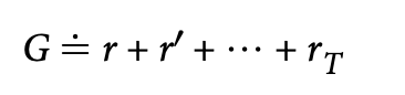
Mathematical representation of Return

Sometimes the final time step may go up to infinity. For example, investing your time studying or exercising doesn’t provide immediate payoffs — the benefits accumulate gradually and are realized over time. To quantify such future rewards, and mitigate against the explosive power of infinity, RL uses the concept of discounting.

The discounted reward (or discounted return), denoted by G, is defined mathematically as:

Discounter return

• r​: Reward at step t.
• γ (Gamma): Discount factor (0 ≤ γ ≤ 1), indicating the importance of future rewards. If γ=0, the agent focuses solely on immediate rewards. As γ approaches 1, the agent increasingly values future rewards. γ typically ranges between 0.9 and 0.99.

Discounting ensures finite sums.

Predicting Rewards

State-Value Functions

The state-value function for a policy, Vπ(s), predicts the expected return with respect to each state s, following policy π. Mathematically:

State-value function

Breaking Down the State-Value Function:

• Vπ(s): The value of state s under policy π.
• Eπ[G|s]: The expected value of the return given a current state, assuming the agent follows policy π.

This expected value can be calculated in many ways, but the simplest is to simply average over all the observed rewards. Also if you notice, you can only calculate the expected return if you already have a policy. But the equation above is meant to help you quantify the performance of a policy. This is a classic chicken and egg problem that RL solves by starting randomly and iterating to find an improvement.

It’s essentially saying: “If I consistently follow this policy, what’s the return, from a state, on average”

To better understand this, let’s consider a simple elevator system. The elevator can move between 5 floors, with the first floor as the lowest level (penalty state) and the fifth floor as the top level (goal state). The elevator must reach the goal state (5th floor) while avoiding the first floor, which results in a penalty.

Problem Definition

• Floors: The elevator operates in a 5-floor building.
• Starting Position: The elevator starts at floor 2.
• Goal Position (Reward State): The 5th floor (+10 reward).
• Penalty State: The 1st floor (−5 penalty).
• Valid States: Floors 2 to 4 are non-terminal states where the elevator can move up or down.
• Actions:
• Move up (+1 floor).
• Move down (−1 floor).
• Strategy/Policy: The elevator randomly chooses to move up or down at each step.

Initialize value_sum[floors] = 0
Initialize n_hits[floors] = 0
Set number_of_episodes = 1000

FOR each episode:
    Initialize position = starting_floor (floor 2)
    Store visited_positions = []

    WHILE True:
        Append position to visited_positions

        IF position is terminal:
            Break

        Update position using random strategy:
            IF random_value > 0.5:
                Move UP (+1 floor)
            ELSE:
                Move DOWN (-1 floor)

    Compute reward(position):
        IF position == goal_floor (5th floor):
            reward = +10
        ELSE IF position == penalty_floor (1st floor):
            reward = -5
        ELSE:
            reward = 0

    Update value estimates:
    FOR each floor in visited_positions:
        value_sum[floor] += reward
        n_hits[floor] += 1

    Compute and print expected value estimates:
        expected_value[floor] = value_sum[floor] / n_hits[floor]

    PRINT expected_action values for episode that are multiples of 100

The expected_value should evolve over time as more episodes are processed:

[Episode 100] Estimated Values: [nan, -3.50, 2.00, 5.00, 8.00, 10.00]
[Episode 200] Estimated Values: [nan, -4.00, 1.50, 5.50, 8.50, 10.00]
...
[Episode 500] Estimated Values: [nan, -4.50, 0.80, 5.80, 9.20, 10.00]
[Episode 1000] Estimated Values: [nan, -5.00, 0.50, 6.00, 9.50, 10.00]

• The goal floor (5th) stabilizes around 10.0, as it always yields +10.
• The penalty floor (1st) stabilizes around −5.0, as it always gives −5.
• The intermediate floors (2nd to 4th) take expected values based on their probability of reaching the goal or penalty state.

The expected_value represent the “Goodness” of a state. Higher values mean states closer to reaching the goal. Lower values mean states closer to penalties. The algorithm learns by experience. Initially, state values are uninitialized. Over time, the algorithm refines the value function based on observed transitions. Therefore, if we replace random movement with a policy that maximizes expected return, we get optimal control. Example: If an agent knows floor 4 has a value of 9.5, it should always move up instead of randomly choosing up/down.

Action-Value Functions

However, states alone don’t always tell the full story. What if different actions in the same state lead to vastly different outcomes? Action-Value Function captures this nuance.

The Action-Value Function predicts the expected reward from choosing a particular action a in a given state s, and then subsequently following policy π:

Notice the subtle yet crucial difference from the State-Value Function. Here, we’re explicitly evaluating the action, not just the state.

Using the problem which was used earlier, now we track the actions and explore both states and actions.

Initialize value_sum[state, action] = 0  # Store total reward per (state, action)
Initialize n_hits[state, action] = 0  # Count state-action visits

Define function reward(position):
    IF position == goal_floor:
        RETURN reward_goal
    ELSE IF position == penalty_floor:
        RETURN reward_penalty
    RETURN 0

Define function is_terminal(position):
    RETURN position == goal_floor OR position == penalty_floor

Define function strategy():
    RETURN +1 IF random_value > 0.5 ELSE -1  # Move UP (+1) or DOWN (-1)

Define function action_value_mapping(action):
    RETURN 0 IF action == -1 ELSE 1  # Map DOWN to index 0, UP to index 1

FOR each episode:
    Initialize position = starting_floor
    Initialize action = strategy()
    Store visited_positions_actions = []

    WHILE True:
        Append (position, action) to visited_positions_actions

        IF is_terminal(position):
            BREAK  # Stop if in terminal state

        # Update position using strategy
        position += strategy()

        # Ensure it stays within valid floors
        position = max(1, min(num_floors, position))

    Compute episode reward = reward(position)

    FOR (pos, act) in visited_positions_actions:
        value_sum[pos, action_value_mapping(act)] += episode_reward
        n_hits[pos, action_value_mapping(act)] += 1

    Compute expected action values:
        expected_action_values[state, action] = value_sum[state, action] / n_hits[state, action]

    PRINT expected_action values for each episode

Similarly the results are like:

[Episode 100] Expected Action Values:
DOWN: [ nan, -3.50, 2.00, 5.00, 8.00, 10.00]
UP:   [ nan,  0.00, 5.00, 5.00, 5.00, 10.00]

[Episode 500] Expected Action Values:
DOWN: [ nan, -4.50, 0.80, 5.80, 9.20, 10.00]
UP:   [ nan,  0.50, 5.00, 5.00, 5.00, 10.00]

[Episode 1000] Expected Action Values:
DOWN: [ nan, -5.00, 0.50, 6.00, 9.50, 10.00]
UP:   [ nan,  1.00, 5.00, 5.00, 5.00, 10.00]

Why Action-Value (Q) is Important?

Instead of just knowing the value of a state, the agent now knows which action is best at each state. This allows for policy improvement by selecting the action with the highest expected return.

Since we now track state-action pairs, learning takes longer because we need to visit all actions sufficiently. Initially, some actions might have NaN values due to insufficient exploration.

Comparison with State-Value Function

State-Value Function V(s): Estimates how good each state is.

Action-Value Function Q(s,a): Estimates how good each action at a given state is.

Advantage of Q-values: The agent doesn’t have to figure out how to reach better states — it can simply pick the best action directly!

Evaluating and Improving Policies

The core of RL lies in policy evaluation and improvement:

• Policy Evaluation: Assessing the current policy by calculating state-value functions.
• Policy Improvement: Using value-function estimates to guide the agent toward better actions.

This iterative loop is fundamental:

1. Start with a policy (possibly random initially).
2. Evaluate the policy by calculating Vπ(s) or Qπ​(s,a).
3. Improve policy based on these values, choosing actions leading to states with higher predicted values.
4. Repeat until you reach an optimal policy, where no further improvement is possible.

Thus, value functions and discounted rewards serve as vital tools for iterative policy improvement.

What is an Optimal Policy?

An optimal policy, denoted as π∗, is a strategy that yields the highest expected return (cumulative reward) when followed consistently. It’s the “best possible plan” an agent can use to navigate an environment.

Optimal Value Functions

An optimal policy is associated with two critical functions:

Optimal State-Value Function, V∗(s):

Represents the highest expected return achievable from a particular state, assuming you always follow the optimal policy thereafter.

Optimal Action-Value Function, Q∗(s,a):

Represents the highest expected return achievable from a particular state-action pair, assuming you always follow the optimal policy afterward.

These two functions contain the same essential information, just presented at different resolutions:

• V∗(s) is like a bird’s-eye view of the best possible outcomes from states.
• Q∗(s,a) gives a detailed, action-level view — helping agents pick specific optimal actions.

The Bellman Optimality Equation formally captures the relationship between these two functions. The simplified form of this equation is:

Optimal Value Function

In simple terms, the optimal value for a state is equal to choosing the best possible action (the action with the highest expected reward) in that state.

What does this mean practically? At each step, if you consistently pick the action that maximizes expected rewards, you’ll achieve the optimal cumulative return.

Why Does Choosing the Highest Reward Always Work?

At first glance, the Bellman equation might seem overly simplistic or even counterintuitive — what if higher rewards exist elsewhere?

The key insight is:

• Optimal value functions and policies assume complete knowledge (or at least accurate predictions) of future rewards.
• Therefore, when choosing the action with the highest action-value at any state, the algorithm has already considered all future possibilities, including moving toward better states later.

This means your action-value function inherently encodes the value of moving towards more rewarding states later on. Thus, repeatedly selecting the action with the highest estimated return is inherently optimal.

Conclusion

• Discounted rewards help the agent balance immediate and future outcomes, controlling how much importance is placed on future rewards through the discount factor γ.
• State-value functions (Vπ(s)) let us evaluate how effective a given policy is by calculating the expected long-term reward starting from a given state.
• Action-value functions (Qπ(s,a)), or Q-functions, refine this understanding by quantifying how valuable specific actions are within states, making it possible to choose optimal decisions.
• Ultimately, an optimal policy (π∗) emerges from consistently choosing actions that lead to states with the highest expected returns.

Together, these concepts form the mathematical backbone of effective decision-making in RL, enabling agents to systematically evaluate their actions, optimize strategies, and adapt dynamically to complex environments.