How to train a Masked Language Model

If you’re reading this, chances are you’re familiar with Large Language Models (LLMs). By now, nearly everyone has heard of these groundbreaking models and their seemingly magical capabilities. However, for the curious minds out there, LLMs aren’t simply a mystical black box that conjures up text, images, or audio. In reality, LLMs come in various forms, each tailored to specific tasks, often leveraging the encoder-decoder architecture of transformers — sometimes partially, sometimes fully.

Before diving deeper into the intricacies, let’s first explore the fundamental process of training an LLM. For the purpose of this article, we’ll focus on how LLMs are trained using textual data.

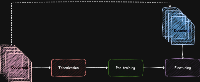
basic flow of LLM training

As illustrated in the figure above, training an LLM involves preparing the textual documents you intend to use. The process begins with tokenization, followed by pre-training the model, and finally fine-tuning it for specific tasks such as classification, text generation, or regression. In this article, we’ll focus on the tokenization and pre-training steps, leaving the fine-tuning discussion for a future piece.

But hold on — what exactly is a Masked Language Model (MLM)? So far, we’ve only discussed Large Language Models (LLMs). MLM plays a critical role in the pre-training phase, but before diving into that, let’s briefly explore the tokenization step.

Tokenization

Imagine you have a massive text corpus in English. Since machine learning models cannot process raw text directly, we need to convert it into a numerical format that mathematical algorithms can understand. In traditional NLP models like TF-IDF, LSTM, or Word2Vec, each word is treated as a single token, which is then assigned a numerical representation.

In the case of Large Language Models (LLMs), tokenization becomes more nuanced and plays a critical role in ensuring efficient and effective text representation. Three popular tokenization techniques used in LLMs are:

• WordPiece — Breaks words into smaller subword units, ensuring rare words are split into more common components while maintaining their semantic meaning.
• Byte Pair Encoding (BPE) — Uses a frequency-based approach to merge characters or subwords iteratively, creating a vocabulary of subword tokens.
• SentencePiece (SPM) — Works independently of language-specific rules and can handle text at the character, subword, or word level, making it more versatile for multilingual corpora.

Each LLM architecture typically employs a specific tokenization technique:

• BERT relies on WordPiece tokenization.
• RoBERTa adopts BPE for its flexibility and efficiency.
• LLAMA utilizes SentencePiece, especially suited for diverse and multilingual datasets.

Why these particular choices? The reasons often relate to the trade-offs between vocabulary size, computational efficiency, and the specific design goals of the model. While this article won’t delve deeper into the mechanics of each tokenization method, it’s crucial to understand their importance.

When training an LLM, selecting the appropriate tokenizer and ensuring it is aligned with your data is essential. This step guarantees that the model can interpret and process your input effectively. While tokenization is a foundational aspect of training, our primary focus in this article will be on the pre-training phase, with tokenization serving as the preliminary step.

Pre-Training

Pre-training a model involves training a base model in an unsupervised manner to grasp the semantics and structure of your dataset. This step is foundational because it enables the model to develop a deep understanding of the underlying patterns in your data, even when most of it is unlabelled.

For example, consider a massive corpus of software logs, primarily unlabelled, that you wish to use for various tasks such as defect classification or configuration categorization. You can pre-train a model like RoBERTa on this corpus using Masked Language Modelling (MLM) in an unsupervised fashion. Once pre-trained, this model serves as a robust base for fine-tuning on downstream tasks, such as building classification models with your labelled data.

There are three primary pre-training methods, each suited to specific tasks and model architectures:

1. Masked Language Modelling (MLM) Used in models like BERT and RoBERTa, this method involves masking a portion of the input tokens and training the model to predict the missing words based on their context. This approach helps the model develop a deep contextual understanding of language.
2. Causal Language Modelling (CLM) Employed in autoregressive models like GPT, CLM trains the model to predict the next word in a sequence. This method is ideal for tasks requiring sequential generation, such as text completion and language translation.
3. Permutation Language Modelling (PLM) Used in models like XLNet, this technique takes a novel approach by considering all possible permutations of word order within a sequence during training. This enhances the model’s ability to understand bidirectional and autoregressive contexts simultaneously.

Choosing the right pre-training method depends on the nature of your dataset and the tasks you aim to accomplish. Pre-training provides a versatile foundation that can be tailored to a variety of applications through fine-tuning, enabling more efficient and effective use of labelled data for specific tasks.

Below is a summary of each type:

Summary of MLM, CLM and PLM

Depending on the model type (and the task), one would select which type of pre-training is required. For e.g., the task at hand for us is to classify software logs and this task belongs to the Encoder part of the transformer architecture, for which we can use models like BERT, RoBERTA or T5(encoder) and these models can be pre-trained as MLM. For our article we will use RoBERTA.

Let’s get into training the RoBERTA as MLM. We start with installing and importing all the pre-requisites.

!pip install Transformers

import os
from pathlib import Path
from tokenizers import ByteLevelBPETokenizer
from transformers import RobertaConfig
from transformers import RobertaTokenizer
from transformers import RobertaForMaskedLM
from transformers import LineByLineTextDataset
from transformers import DataCollatorForLanguageModeling
from transformers import Trainer, TrainingArguments
from transformers import pipeline

In this example we are dealing with .txt file(s). So get all the content either in one single file or all the files in a single directory. I will not be going through any cleaning/ pre-processing steps in this example and will treat the raw data as it is.

The first key step is to train our own tokenizer on the data we have at hand. The reason behind this is that since we are training the Model from scratch, our model doesn’t have any information of the language or the tokens and we will have to train and use our own tokenizer so that the model can use that information when encoding the data.

# Get the list of all .txt files
paths = [str(x) for x in Path('.').glob("**/*.txt")]

# initialize a tokenizer
tokenizer = ByteLevelBPETokenizer()
# Train the tokenizer
tokenizer.train(
    files=paths, 
    vocab_size=52_000, 
    min_frequency=2, 
    special_tokens = [
        "<s>",
        "<pad>",
        "</s>",
        "<unk>",
        "<mask>"
    ])
token_dir = '/content/RoBERTA'
if not os.path.exists(token_dir):
  os.makedirs(token_dir)
tokenizer.save_model('RoBERTA')

As mentioned previously, RoBERTA uses BPE tokenizer. Hence, we initialize a BPE tokenizer and train it on the text corpus we have and save the tokenizer vocab and merges files locally. You can set the vocab_size of the tokenizer as per your data. For s/w logs, we can also add special tokens like <IP_ADDR> or <HEX> and replace the these tokens with the actual IP addresses and HEX values in the raw text to make the data much cleaner for the model to learn from.

['RoBERTA/vocab.json', 'RoBERTA/merges.txt']

The next step is to initialise our RoBERTA model

# Define the configuration of the model
config = RobertaConfig(
    vocab_size=52_000,
    max_position_embeddings=514,
    num_attention_heads=12,
    num_hidden_layers=6,
    type_vocab_size=1
)

# Initialise RobertaTokenizer using the files saved
tokenizer = RobertaTokenizer.from_pretrained(
    "./RoBERTA",
    max_length = 512
)

# Initialise the model
model = RobertaForMaskedLM(config=config)

The configuration of the model can be modified depending on the analysis of data and other requirements. Once model is successfully initialised, we can review the model parameters just by print(model)

RobertaForMaskedLM(
  (roberta): RobertaModel(
    (embeddings): RobertaEmbeddings(
      (word_embeddings): Embedding(52000, 768, padding_idx=1)
      (position_embeddings): Embedding(514, 768, padding_idx=1)
      (token_type_embeddings): Embedding(1, 768)
      (LayerNorm): LayerNorm((768,), eps=1e-12, elementwise_affine=True)
      (dropout): Dropout(p=0.1, inplace=False)
    )
    (encoder): RobertaEncoder(
      (layer): ModuleList(
        (0-5): 6 x RobertaLayer(
          (attention): RobertaAttention(
            (self): RobertaSdpaSelfAttention(
              (query): Linear(in_features=768, out_features=768, bias=True)
              (key): Linear(in_features=768, out_features=768, bias=True)
              (value): Linear(in_features=768, out_features=768, bias=True)
              (dropout): Dropout(p=0.1, inplace=False)
            )
            (output): RobertaSelfOutput(
              (dense): Linear(in_features=768, out_features=768, bias=True)
              (LayerNorm): LayerNorm((768,), eps=1e-12, elementwise_affine=True)
              (dropout): Dropout(p=0.1, inplace=False)
            )
          )
          (intermediate): RobertaIntermediate(
            (dense): Linear(in_features=768, out_features=3072, bias=True)
            (intermediate_act_fn): GELUActivation()
          )
          (output): RobertaOutput(
            (dense): Linear(in_features=3072, out_features=768, bias=True)
            (LayerNorm): LayerNorm((768,), eps=1e-12, elementwise_affine=True)
            (dropout): Dropout(p=0.1, inplace=False)
          )
        )
      )
    )
  )
  (lm_head): RobertaLMHead(
    (dense): Linear(in_features=768, out_features=768, bias=True)
    (layer_norm): LayerNorm((768,), eps=1e-12, elementwise_affine=True)
    (decoder): Linear(in_features=768, out_features=52000, bias=True)
  )
)

We can modify the model parameters as per our need. For smaller datasets and smaller models we can reduce the number of attention heads and layers for e.g.

The next step is to prepare the data for the model. For this example I am using an open source english text data of about 1.3 MB in size. The data can be prepared by either using LineByLineTextDataset or constantlengthdataset from huggingface and the tokenizer trained earlier on our dataset.

dataset = LineByLineTextDataset(
    tokenizer = tokenizer,
    file_path = './logs.txt',
    block_size = 128
)

As a result we convert the data into multiple chunks of tokenized data as shown below

{'input_ids': tensor([   0,  322, 4366,  305,   16,  419, 9317,   18,  703, 7414, 1006,  267,
          2668,  321,  267,    2])},
 {'input_ids': tensor([   0, 6643, 5099,   16,  327,  300,   16,  280,  267, 2047, 1127,  270,
          1897,   16,  345,    2])},
 {'input_ids': tensor([   0, 1433,  489, 3171,  288,  267, 2099, 1538,  270,  267, 3476,  781,
          7871,   42,   16,  267,    2])},

The next step in terms of data is to use Data Collator to batch the data and prepare it for Masked Language Modelling

data_collator = DataCollatorForLanguageModeling(
    tokenizer = tokenizer,
    mlm = True,
    mlm_probability=0.15
)

Here we are masking 15% of the data for the model to learn and predict

DataCollatorForLanguageModeling(
tokenizer=RobertaTokenizer(
name_or_path='./RoBERTA', 
vocab_size=9943, 
model_max_length=1000000000000000019884624838656, 
is_fast=False, 
padding_side='right', 
truncation_side='right', 
special_tokens={
'bos_token': '<s>', 
'eos_token': '</s>', 
'unk_token': '<unk>', 
'sep_token': '</s>', 
'pad_token': '<pad>', 
'cls_token': '<s>', 
'mask_token': '<mask>'}, 
clean_up_tokenization_spaces=False),  
added_tokens_decoder={
 0: AddedToken("<s>", rstrip=False, lstrip=False, single_word=False, normalized=True, special=True),
 1: AddedToken("<pad>", rstrip=False, lstrip=False, single_word=False, normalized=True, special=True),
 2: AddedToken("</s>", rstrip=False, lstrip=False, single_word=False, normalized=True, special=True),
 3: AddedToken("<unk>", rstrip=False, lstrip=False, single_word=False, normalized=True, special=True),
 4: AddedToken("<mask>", rstrip=False, lstrip=True, single_word=False, normalized=False, special=True),
}, 
mlm=True, 
mlm_probability=0.15, 
pad_to_multiple_of=None, 
tf_experimental_compile=False, 
return_tensors='pt')

Final step is to provide all the above information to the model and train the model

training_args = TrainingArguments(
    output_dir = './RoBERTA',
    overwrite_output_dir=True,
    num_train_epochs=2,
    per_device_train_batch_size=64,
    save_steps = 10_000,
    save_total_limit=2,
    report_to="none"
)

trainer = Trainer(
    model=model,
    args=training_args,
    data_collator= data_collator,
    train_dataset=dataset
)
trainer.train()
trainer.save_model("./RoBERTA")

Once the model has been trained, we can verify what the model has learned from the training. I am not yet aware of any metrics that can be used to evaluate MLM performance except monitoring the training loss.

fill_mask = pipeline(
    "fill-mask",
    model='./RoBERTA',
    tokenizer="./RoBERTA"
)
fill_mask("the weather is <mask>")

And the output will be as shown below. The model predicts “,” as the next token. Which in reality is not what we expect but can be improved by further changes in the training args.

Device set to use cuda:0
[{'score': 0.06988143175840378,
  'token': 16,
  'token_str': ',',
  'sequence': 'the weather is,'},
 {'score': 0.06902889907360077,
  'token': 270,
  'token_str': ' of',
  'sequence': 'the weather is of'},
 {'score': 0.04994117468595505,
  'token': 267,
  'token_str': ' the',
  'sequence': 'the weather is the'},
 {'score': 0.03335319459438324,
  'token': 18,
  'token_str': '.',
  'sequence': 'the weather is.'},
 {'score': 0.022917794063687325,
  'token': 280,
  'token_str': ' in',
  'sequence': 'the weather is in'}]

Conclusion

In this article, we explored how to pre-train RoBERTa as a Masked Language Model (MLM) using custom data. By doing so, the model learns to understand the semantic structure and patterns within the dataset, creating a robust foundation for various applications.

Once pre-trained, this model can be seamlessly adapted for downstream tasks. For instance, it can be fine-tuned for classification tasks using specialized architectures like RobertaForSequenceClassification, enabling it to perform efficiently with labelled data for tasks such as defect categorization, sentiment analysis, or other classification problems.