Capacity aware A/B/n Testing Design

How to design a capacity-aware experiment to find the best retention offer

…continued from *A Practical Guide for Designing Rigorous Retention Experiments *…

So, your churn prediction model is a success. It’s running, it’s accurate, and it’s dutifully spitting out a list of high-risk customers every week. Congratulations.

Now what?

The business, of course, doesn’t just want to know who is leaving; they want to stop them. Your marketing director is ready to act. They’ve come up with three new “offers” to win back these at-risk customers:

• Offer 1: A 10% discount for 12 months.
• Offer 2: A one-time “premium feature” unlock.
• Offer 3: A personal “customer success” call.

Which one works best? Which one provides the highest lift in renewal rates? And, most importantly, what if you can’t offer them to everyone?

This is a classic causal inference problem. We can’t just “spray and pray.” We need to design a controlled experiment — an A/B/n test — to measure the true “lift” of each offer against a “control” group that gets nothing.

But there’s a twist. In the real world, resources are finite. Your marketing director tells you the outbound call center (which delivers these offers) has a total capacity of 1,000 calls for this campaign.

This is a capacity-aware design problem. We need to find the best offer, but we must do so within our budget.

Let’s walk through how to design this experiment from a data science perspective, from statistical power to the final audience list.

Step 1: Statistical Power & Our “Ideal” Sample Size

Before we can even think about our 1,000-call limit, we must answer a more fundamental question: What is the minimum number of people we need in each group to detect a meaningful change?

If we use too few people, we might get “lucky.” We might see a 5% lift that was just random noise, or worse, we might miss a real, 5% lift because our sample was too small to detect it.

This is called Statistical Power Analysis. We need to define four things:

1. Baseline Conversion Rate (p1): What percentage of “high-risk” customers renew anyway, even if we do nothing? Let’s say we look at historical data and find it’s 80%.
2. Minimum Detectable Effect (MDE): What is the smallest lift we care about? The business decides a 5 percentage point increase (i.e., from 80% to 85%) is the minimum that would justify the cost of the offer.
3. Alpha (α): Our risk of a false positive (a Type I Error). We’ll use the standard 0.05.
4. Power (1-β): Our chance of “detecting” a real effect (avoiding a false negative). We’ll use the standard 0.80.

With these four values, we can calculate our required sample size per group.

A Quick Glossary of Terms

• Effect Size: The magnitude of the difference we want to measure. For proportions, we use Cohen’s h, which is a standard way to measure the “distance” between two proportions (like 40% and 45%).
• Type I Error (α): A “false positive.” We conclude an offer has an effect, but it actually doesn’t. We set this risk at 5%.
• Type II Error (β): A “false negative.” The offer does have an effect, but our test fails to detect it. We set this risk at 20% (giving us 80% Power).
• Arm: A distinct group in our experiment (e.g., Control, Offer 1, Offer 2, Offer 3).

Note:

Statsmodels expects an effect size, not raw pp lift. For a two-group proportion test they use Cohen’s h:

We feed h, sample allocation (control vs offer), and α (with multiplicity adjustment) into the power engine to get:

• Power (chance to detect that lift), or
• MDES (smallest lift detectable at target power), or
• Sample size needed for a chosen MDES/power.

What is “proportion effect” a.k.a. Cohen’s h?

It’s a standardized way to express a change in a proportion (like renewal rate) that automatically adjusts for how easy or hard it is to detect changes at different baselines:

e.g., start with a baseline renewal rate p0 (e.g., 60%) and a new rate p1 (e.g., 63%).

The plain change is percentage-point lift Δ = p1 — p0 (here, +3 pp).

Cohen’s h converts both proportions through a variance-stabilizing transform and takes the difference: h = 2 arcsin √p1 — 2 arcsin √p0

Why not just use percentage points?

Because the same pp lift is not equally hard to detect at different baselines:

Around 50%, outcomes are noisiest → you need more sample.

Near 0% or 100%, outcomes are less noisy → the same pp lift is easier to detect (but “headroom” limits near 100%).

h automatically accounts for that. It’s a signal-to-noise version of the lift.

Percentage points tell you how much the needle moves.

• Cohen’s h tells you how big that move is relative to the background noise at a baseline.
• Bigger h → easier to detect → higher power (for the same N). For the same pp lift, h is larger near very high/low baselines than around 50%, reflecting the lower noise there.

N. B.: We always report the business-friendly pp lift, but we use h under the hood to size tests correctly.

Step 2: The Python Code to Find Our Sample Size

We’ll use standard Python libraries to do this. scipy.stats helps us with basic statistics, and statsmodels has a powerful function for power analysis.

First, let’s import our tools.

import numpy as np
import pandas as pd
from scipy.stats import norm
from statsmodels.stats.power import zt_ind_solve_power
from statsmodels.stats.proportion import proportions_ztest

Now, let’s write a function to calculate the required sample size. This function will convert our two proportions into an “effect size” (Cohen’s h) and then use zt_ind_solve_power to find the number of observations (nobs1) we need.

def solve_mde(baseline_conversion, mde, alpha, power):
    """
    Calculates the required sample size per group for a test of proportions.

    Args:
        baseline_conversion (float): The conversion rate of the control group.
        mde (float): The minimum detectable effect (e.g., 0.05 for a 5% lift).
        alpha (float): The p-value threshold (Type I error rate).
        power (float): The desired power (1 - Type II error rate).

    Returns:
        int: The required sample size per group.
    """

    # Calculate the two proportions
    p1 = baseline_conversion
    p2 = baseline_conversion + mde

    # Calculate Cohen's h for effect size
    # This is the standard way to measure distance between two proportions
    es = 2 * np.arcsin(np.sqrt(p1)) - 2 * np.arcsin(np.sqrt(p2))

    # Solve for sample size (nobs1)
    # We use 'zt_ind_solve_power' for a two-sample Z-test
    n = zt_ind_solve_power(
        effect_size=es,
        alpha=alpha,
        power=power,
        ratio=1.0,  # We assume equal sample sizes (ratio=1.0)
        alternative='two-sided'
    )

    return int(np.ceil(n))

If you are worried about incremental “lift” in a churn experiment, do you consider one-sided or two-sided test? Why or why not? When you’re looking for an “incremental lift” in a churn experiment, it implies you’re hoping to decrease churn. This might initially suggest a one-sided test, where your hypothesis is specifically that the new intervention will lead to less churn.

However, in most real-world A/B/n tests, especially in churn experiments, it’s generally recommended to use a two-sided test.

Here’s why:

Detection of Negative Effects: While you are hoping for a “lift” (i.e., a decrease in churn), it’s equally, if not more, important to detect if your intervention accidentally increases churn or has no effect. A two-sided test allows you to detect a significant effect in either direction (positive or negative). Unexpected Discoveries: An intervention might have unintended negative consequences that you wouldn’t want to miss. For example, a new feature meant to reduce churn might inadvertently alienate a segment of users, leading to higher churn for them. A one-sided test focused only on reduction would not flag this significant increase. Robustness and Bias: Using a one-sided test requires a strong prior belief that the effect can only go in one direction, or that you truly only care about one direction of effect. If your assumption is wrong, or if you later find yourself looking at the negative results and wishing you had set up a two-sided test, you could be introducing bias. A two-sided test is more robust as it doesn’t commit to a direction beforehand. Industry Standard: Most causal testing frameworks and statistical guidelines recommend two-sided tests as the default because they provide a more comprehensive and unbiased evaluation of the intervention’s impact.

In short, while the primary goal is still an incremental decrease in churn, using a two-sided test provides a more complete and safer statistical analysis by allowing you to detect any significant change, whether it’s a desirable reduction in churn or an undesirable increase in churn.

Let’s run it with our inputs for a hypothetical scenario:

# Our inputs
baseline_conversion_rate = 0.85  # 85%
mde = 0.05                       # 5% lift (to 90%)
alpha = 0.05                     # 5% false positive rate
power = 0.80                     # 80% chance to detect a real effect

# Calculate the ideal sample size
n_required = solve_mde(baseline_conversion_rate, mde, alpha, power)

print(f"Required sample size per group (n): {n_required}")

This gives us our “ideal” number for sample-size:

Required sample size per group (n): 681

In a perfect world, we would need 681 customers in each of our experiment groups to reliably detect a 5% lift on a baseline of 85% for an 80% powered experiment.

Step 3: The Real-World Constraint (Factoring in Capacity)

Now, we bring in the business constraint.

• Groups: We have 4 “arms” (1 Control + 3 Offers)
• Ideal Sample Size: 681 per group
• Total Capacity Needed: 4 * 681= 2,724
• Total Capacity Available: 1,000

We have a shortfall. We can’t meet the ideal sample size. This is a critical moment for a data scientist. We must document this discrepancy and explain the trade-off to the marketing director.

Here’s how we can script this check and find our actual sample size per group:

# Our experiment and capacity parameters
n_groups = 4  # 1 Control + 3 Offers
total_capacity = 1000

# Check if we have enough capacity
total_needed_capacity = n_groups * n_required

if total_capacity < total_needed_capacity:
    print(f"Warning: Total capacity ({total_capacity}) is less than required ({total_needed_capacity}).")
    print("The experiment may be underpowered to detect a {mde*100}% lift.")

    # We must reduce our sample size to fit the capacity
    sample_size_per_group = total_capacity // n_groups
    print(f"New sample size per group will be: {sample_size_per_group}")
else:
    sample_size_per_group = n_required
    print(f"Capacity is sufficient. Sample size per group: {sample_size_per_group}")

total_sample_size = sample_size_per_group * n_groups

Warning: Total capacity (1000) is less than required (2724).
The experiment may be underpowered to detect a {mde*100}% lift.
New sample size per group will be: 250

So the experiment is underpowered to detect a 5% lift on a baseline of 85% with 250 observations per group.

The experiment design ultimately needs to answer the question: “what’s the smallest signal we can detect with this design?”

Translated loosely: Statistical power of a causal experiment is about how likely the test is to detect a lift that truly exists: Power = P(reject H₀ | true lift ≥ MDE), where null hypothesis, H₀, is “offer has no lift vs control”

For capacity-constrained (e.g., 250 contacts ), one may fix N and compute the minimum MDE one can detect at 80% power instead. Any change less than MDE fails to register!!

import numpy as np
from statsmodels.stats.power import zt_ind_solve_power

# Existing parameters
baseline_conversion = baseline_conversion_rate  # from previous cells
alpha = alpha                                 # from previous cells
power = power                                 # from previous cells
constrained_sample_size_per_group = sample_size_per_group # from previous cells (250)

p1_transformed = 2 * np.arcsin(np.sqrt(baseline_conversion))

# 2. Solve for the detectable effect size (Cohen's h)
es_detectable = zt_ind_solve_power(
    effect_size=None, # We are solving for effect_size
    nobs1=constrained_sample_size_per_group,
    alpha=alpha,
    power=power,
    ratio=1.0,
    alternative='two-sided'
)

p2_transformed = p1_transformed - es_detectable
p2_detectable = (np.sin(p2_transformed / 2))**2

# 4. Calculate the new Minimum Detectable Effect (MDE)
#    MDE is the absolute difference between p1 and p2
new_mde_absolute = abs(p2_detectable - baseline_conversion)

print(f"With a sample size of {constrained_sample_size_per_group} per group, the new detectable conversion rate (p2) is: {p2_detectable:.4f}")
print(f"The new Minimum Detectable Effect (MDE) in absolute terms is: {new_mde_absolute:.4f} ({new_mde_absolute*100:.2f}%)")

With a sample size of 250 per group, the new detectable conversion rate (p2) is: 0.7505
The new Minimum Detectable Effect (MDE) in absolute terms is: 0.0995 (9.95%)

Since it’s a two-sided test, the new_mde_absolute of 9.95% means that a change of at least 9.95% in either direction from the baseline conversion rate (85%) would be statistically detectable (with the given alpha, power, and sample size).

Let’s break it down with numbers:

• Baseline Conversion Rate (p1): 85% (0.85)
• New Absolute MDE: 9.95% (0.0995)

For a two-sided test, this means:

1. Detectable Decrease: If the true conversion rate decreased by at least 9.95% from the baseline, meaning it drops to 75.05% (0.85–0.0995).
2. Detectable Increase: If the true conversion rate increased by at least 9.95% from the baseline, meaning it rises to 94.95% (0.85 + 0.0995).

Explanation: 
The calculation for p2_detectable (0.7505) happens to solve for one of the 
two scenarios. This is because the zt_ind_solve_power 
function, when solving for effect_size, provides an absolute value. 
When you then perform the back-calculation to get p2_detectable using 
p1_transformed - es_detectable, it mathematically lands on the lower of the 
two possible p2 values given the es_detectable magnitude. If es_detectable 
were applied as p1_transformed + es_detectable, you would get the higher p2 
value.

Regardless of the direction you go (i.e., calculate mde from the fixed group size OR calculate the sample size from a fixed desired mde), the next step is :

Step 4: Final Group Assignment

Now for the final step: creating the audience file. We have our high-risk churn list (let’s say it has 20,000 customers in it) and we need to randomly select 1,000 of them and assign them to our four groups.

Random assignment is crucial to ensure our groups are unbiased.

# 1. Create a mock high-risk customer list (replace with your actual data)
customer_ids = [f"cust_{1000 + i}" for i in range(20000)]
high_risk_customers = pd.DataFrame({'customer_id': customer_ids})

# 2. Shuffle the entire list to ensure randomness
high_risk_customers = high_risk_customers.sample(frac=1).reset_index(drop=True)

# 3. Select only the customers we have capacity for
experiment_audience = high_risk_customers.head(total_sample_size).copy()

# 4. Create the group assignments
group_names = ["Control", "Offer 1", "Offer 2", "Offer 3"]
group_assignments = np.repeat(group_names, sample_size_per_group)

# 5. Shuffle the assignments and add them to the DataFrame
np.random.shuffle(group_assignments)
experiment_audience['group'] = group_assignments

# --- Show the results ---
print("\nFinal Experiment Audience Head:")
print(experiment_audience.head())

print("\nFinal Group Counts:")
print(experiment_audience['group'].value_counts())

This code gives us our final, actionable file for the marketing team. The output confirms our groups are perfectly balanced.

Final Experiment Audience Head:

Final Experiment Audience Head:
  customer_id    group
0   cust_2229  Offer 3
1  cust_15079  Control
2   cust_5994  Offer 3
3  cust_13728  Control
4   cust_4933  Offer 1

Final Group Counts:

Final Group Counts:
group
Offer 3    250
Control    250
Offer 1    250
Offer 2    250
Name: count, dtype: int64

What’s Next?

We’ve done it. We’ve used statistical principles to design an ideal experiment, pragmatically adapted it to a real-world business constraint, and created a clean, randomized, and actionable audience list.

The file experiment_audience is now ready to be delivered to the call center and marketing teams. After the campaign runs, we will join this file with our renewals data, and use the proportions_ztest function we imported to see which, if any, of our offers created a statistically significant lift.

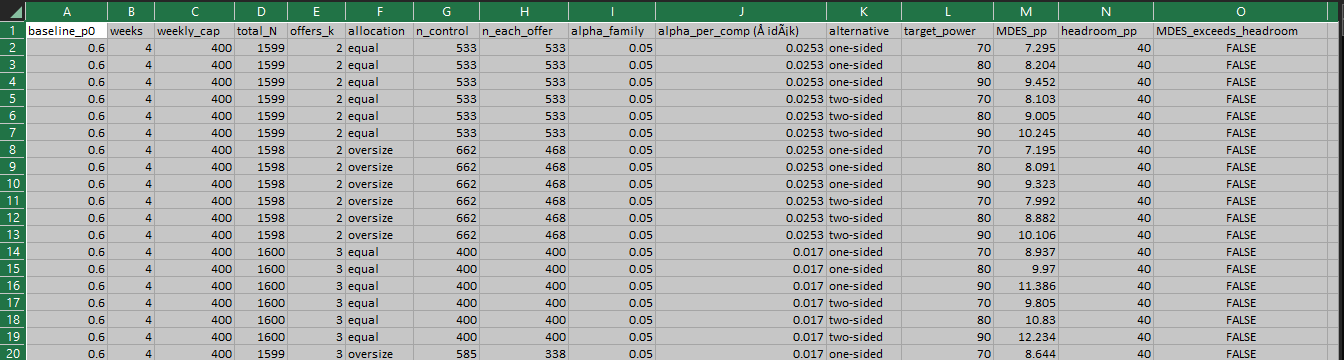
…in the *next post* we parameterize the statistical power calculation for a parallel A/B/n test design so that it outputs a table at varying levels of baseline rate, mdes, powers and sample-sizes