Introduction to LLM Quantization

LLM quantization reduces a model’s memory and computation requirements by storing weights with fewer bits (e.g., 4-bit instead of 16-bit) while maintaining nearly the same performance.

In this blog, we will explore deepseek innovation towards quantization.

1. Mixed Precision Quantization
2. Fine-grained Quantization
3. Increasing accumulation Quantization
4. Mantissa over Exponents
5. Online Qunatization

At first let’s understand what quantization is.

Quantization aims to reduce the precision of a model’s parameters from higher bit-widths (like 32-bit floating point) to lower bit-widths (like 8-bit integers).

Main idea of Quantization is that every parameters in LLM takes a space so, parameters can be represented as FP32 bit,FP16 bit etc.

Main advantage we get is that we reduce the total memory requirements but at the same time we do pay that much heavy price with accuracy of the model.

Of course, accuracy of model slightly reduces because every parameters will be represented with low precision but it is fine in LLM as it doesn’t degrades performance of model that much.

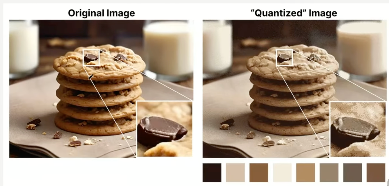
In above figure notice how the zoomed-in part seems more “grainy” than the original since we can use fewer colors to represent it.

The main goal of quantization is to reduce the number of bits (colors) needed to represent the original parameters while preserving the precision of the original parameters as best as possible.

In this blog, we will come across following technical terms:

Common Data Types

FP16

Let’s look at an example of going from 32-bit to 16-bit (called half precision or FP16) floating point:

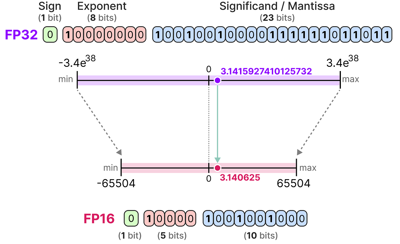
Notice how the range of values FP16 can take is quite a bit smaller than FP32.

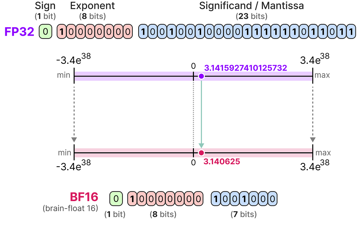
BF16

BF16 (BFloat16) was created to save memory while still handling very large and very small numbers like FP32.

It uses only 16 bits, but keeps a wide value range, making it useful for training and running deep learning models.

INT8

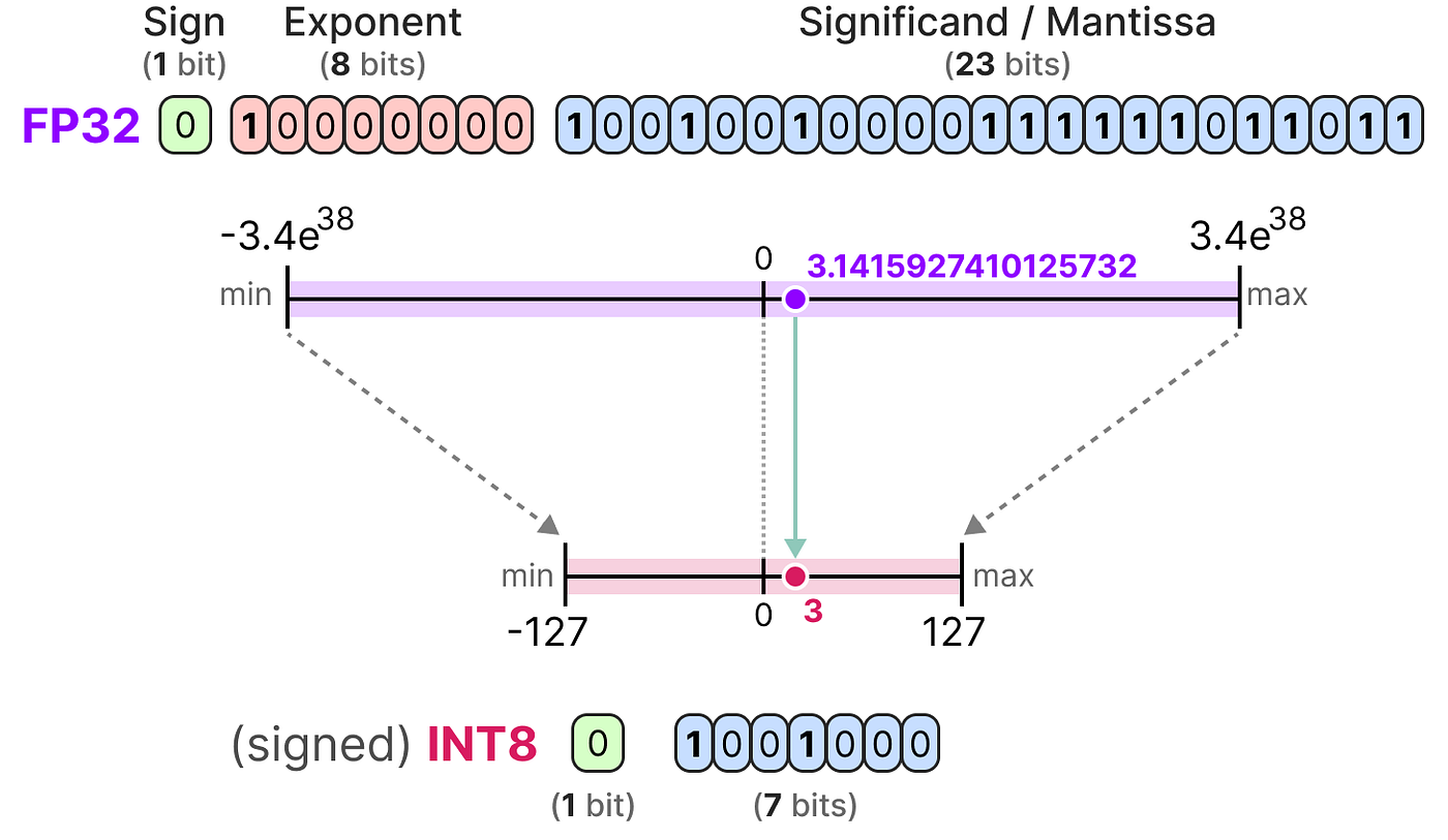
When we reduce precision beyond FP16 or BF16, we move from floating-point numbers to integer formats such as INT8.

For example, converting FP32 to INT8 reduces memory usage by 4× because INT8 uses only 8 bits instead of 32.

To make this possible, the original FP32 values are “squeezed” into a smaller range using a mapping process.

Rather than mapping the entire FP32 range, quantization only maps the actual range of model weights or activations.

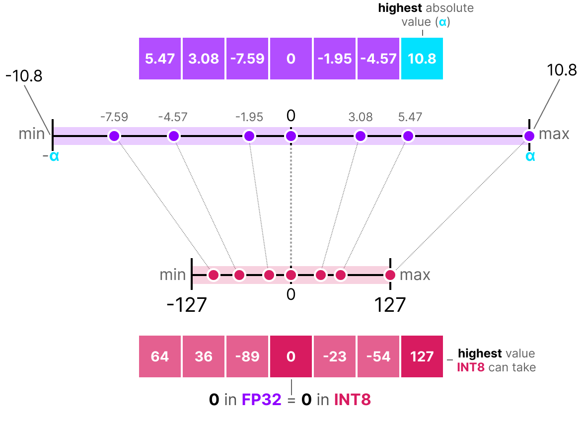
Common methods include symmetric and asymmetric quantization, which linearly transform FP32 values into INT8 while preserving as much information as possible.

When you actually quantize and go from floating point 32 to integer 8, you see the sequence of numbers in floating point 32 and divide all number by highest number(alpha)=10.8 and what you do is that multiply with 127.

Keep in mind divide by highest number and multiply by 127.

Let’s start with major concept how deepseek is implemented.

1. Mixed Precision Quantization

1) Imagine training a simple neural network layer (y = Wx):

→ Input (x): 128 × 1

→ Weights (W): 256 × 128

→ Output (y): 256 × 1

2) Forward propagation (Fprop):

During forward propagation, the output is computed as y = Wx.

To maintain numerical stability, y is initially computed in FP32 and then converted to BF16 for storage.

The weight matrix W is maintained in high precision (BF16 or FP32) but is converted to FP8 on the fly during computation to improve efficiency.

Similarly, the input x is converted from BF16 to FP8 before the matrix multiplication. The computation is therefore performed as

y₍FP32₎ = W₍FP8₎ × x₍FP8₎, where the result is accumulated in FP32 for accuracy and then stored in BF16 to reduce memory usage.

3) Backward propagation:

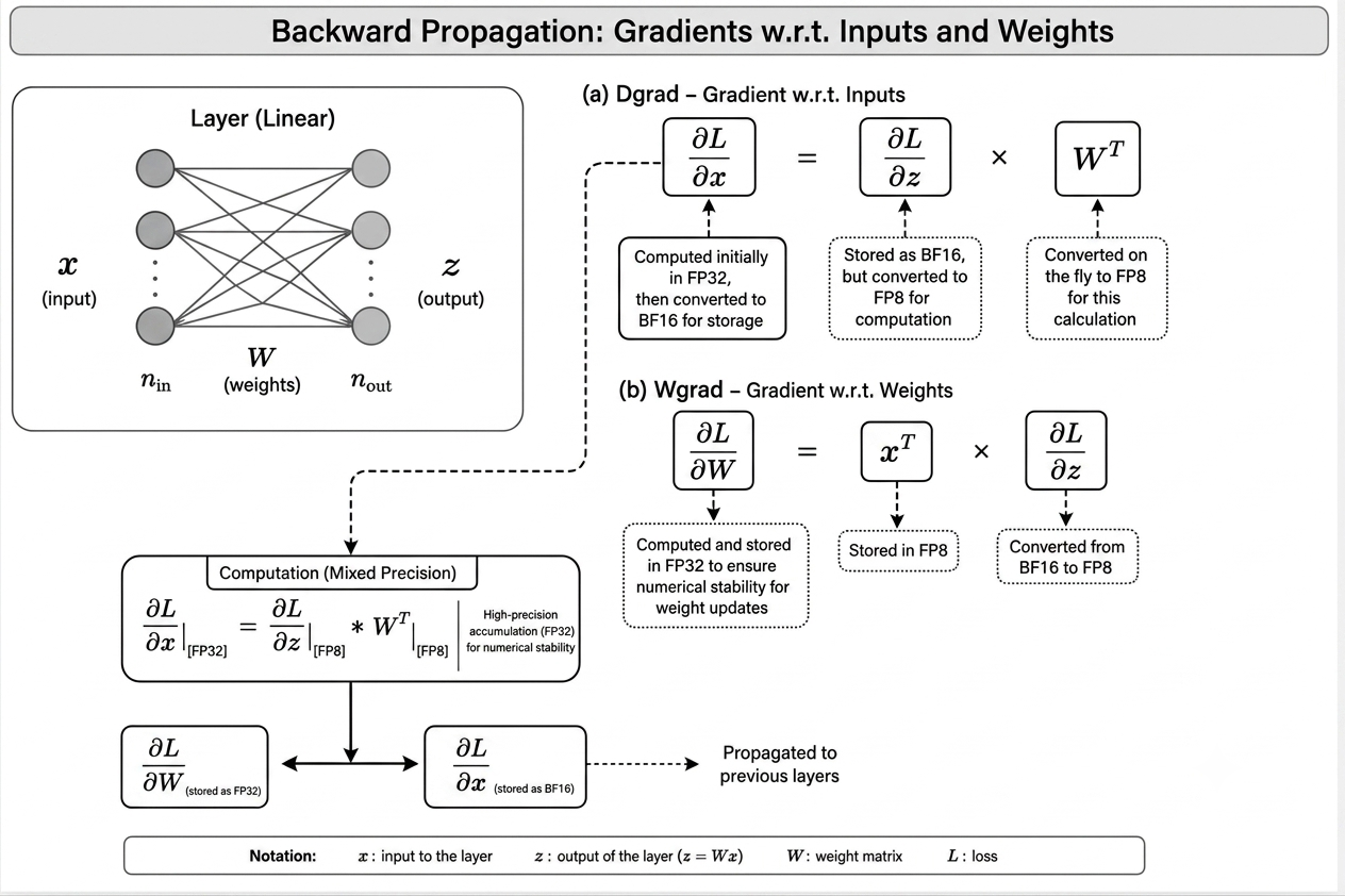
This diagram illustrates backward propagation for a linear layer (z = Wx) using mixed-precision training (FP32, BF16, and FP8).

During backpropagation, two gradients are computed: the input gradient (Dgrad), ∂L/∂x = (∂L/∂z)Wᵀ, which is passed to the previous layer, and the weight gradient (Wgrad), ∂L/∂W = xᵀ(∂L/∂z), which is used to update the model weights.

To improve efficiency, inputs, weights, and gradients are often stored in BF16 and temporarily converted to FP8 during computation, while gradient accumulation is performed in FP32 to maintain numerical stability and training accuracy.

This approach reduces memory usage and computational cost while preserving training quality.

4) Weight Updates(Optimization Step):

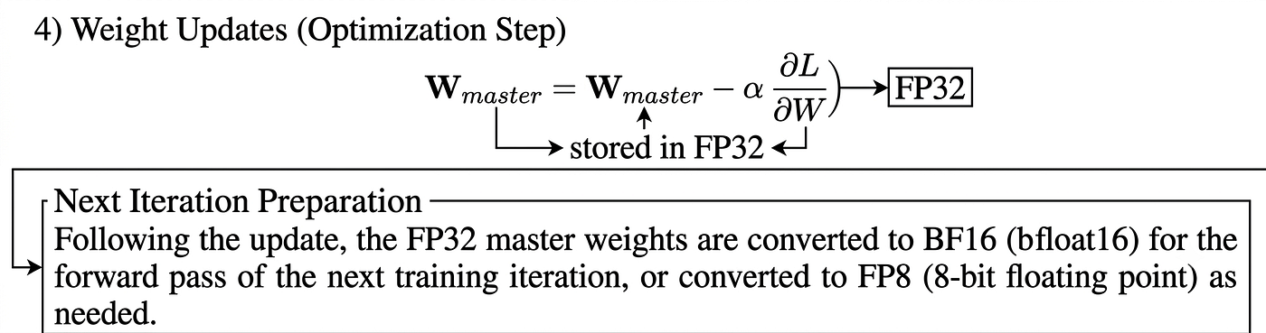
Weight Updates(Optimization Step)

Now, you can understand diagram Mixed Precision Quantization

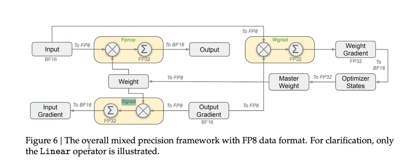
Mixed Precision Quantization

FP8 Precision

1. Significantly reduces computational and memory costs.
2. Provides up to 2× speed improvement compared to BF16 operations.
3. Ideal for computationally intensive GEMM (matrix multiplication) operations.

Higher Precision Retained (FP32/BF16)

While FP8 is used for most computations, some components are highly sensitive to numerical precision and therefore remain in FP32 or BF16. These include:

1. Embedding layers, output heads, gating modules, normalization layers, and attention operators, which require higher precision to maintain model quality.
2. Master weights and optimizer states are typically stored in FP32 to ensure stable and accurate training.Key Idea

This balance between high-precision storage (FP32/BF16) and low-precision computation (FP8) provides the best trade-off between computational efficiency, memory savings, and numerical stability, enabling faster and more efficient training without significantly sacrificing model performance.

2) Fine-grained Quantization:

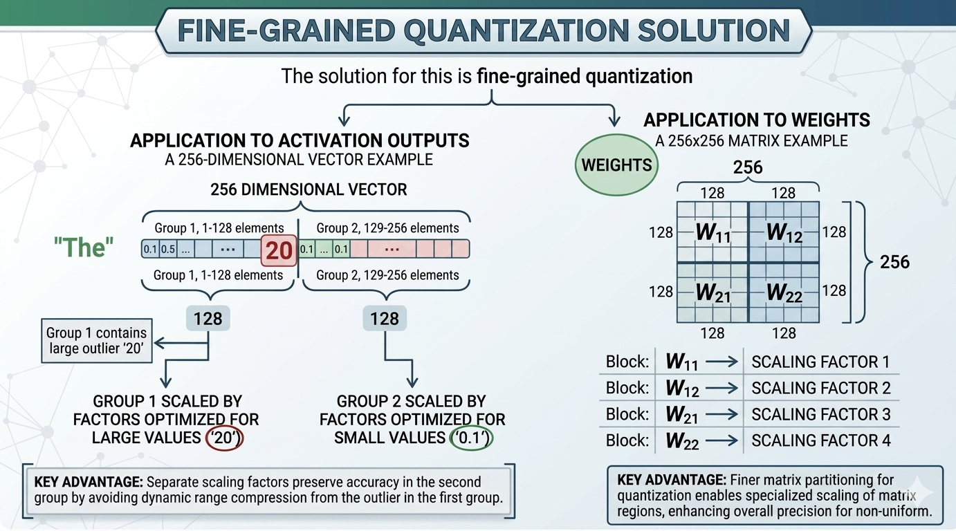
Fine-grained Quantization starts with these scaling solution. You have initial sequence of solution. You take maximum value from sequence divide by it and multiply by 127 if you are converting it to FP8.

When we move to lower-precision formats such as FP8, the number of exponent bits decreases, reducing the range of values that can be represented.

As a result, very large values may cause overflow, while very small values may cause underflow, leading to loss of precision or even becoming zero.

A common solution is to scale the entire tensor based on its largest absolute value so that all values fit within the representable FP8 range.

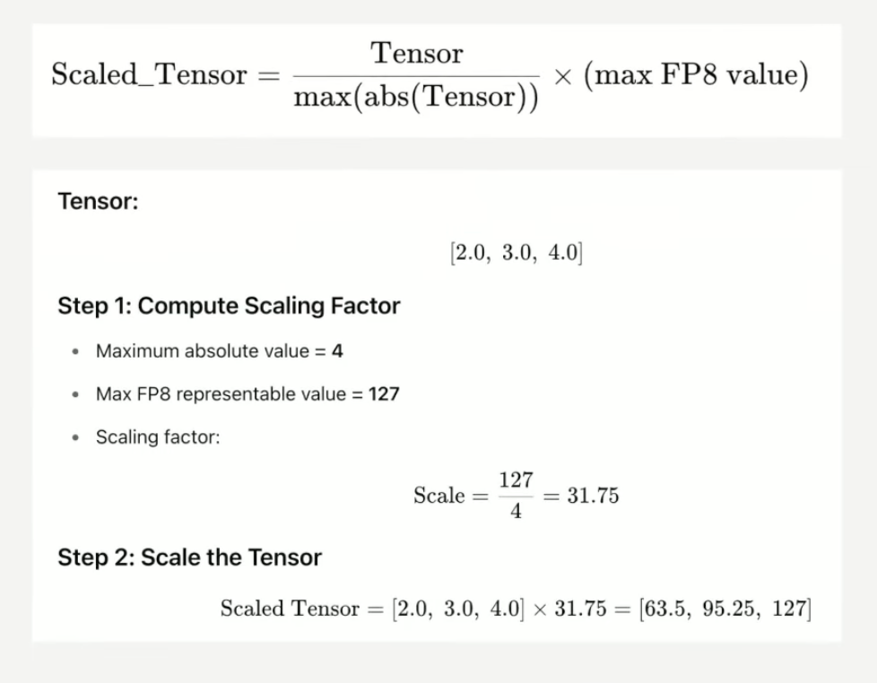
This approach has a weakness. Even a single outlier can drastically reduce the representation accuracy for the whole tensor.

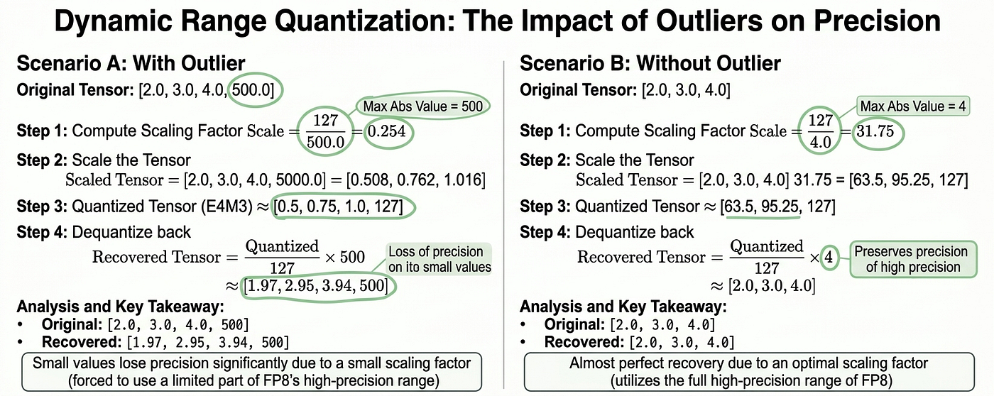
Impact of Outliers on Precision

Fine-Grined Quantization

Fine-grained quantization divides activations and weights into smaller blocks, each with its own scaling factor. This reduces the impact of outliers, preserves accuracy, and improves model performance compared to using a single scale for the entire tensor.

Fine-grained Quantization

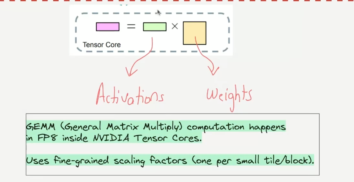
This diagram below shows that matrix multiplication (GEMM), the core operation in neural networks, is performed in FP8 on NVIDIA Tensor Cores using quantized activations and weights.

To maintain accuracy, fine-grained scaling factors are applied to small blocks of data, allowing efficient computation while minimizing quantization errors.

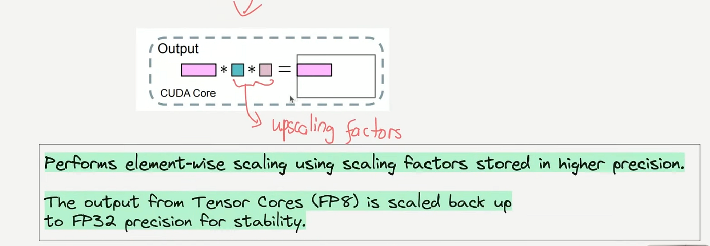
This step in diagram below occurs after the FP8 matrix multiplication is completed on the Tensor Cores.

The FP8 output is multiplied by the stored scaling factors (upscaling factors) on the CUDA Cores to restore its original numerical range.

The result is then converted back to higher precision, typically FP32, which improves numerical stability and reduces the accuracy loss introduced by FP8 quantization.

The diagram below is now easy to understand present in DeepSeek paper.

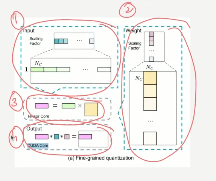
This figure shows fine-grained quantization, where instead of using one scaling factor for the entire tensor, the tensor is divided into small blocks, and each block gets its own scaling factor.

Step 1: Divide into Blocks

• The input activations and weights are split into small groups (blocks) of size N₍C₎.
• Each block has its own scaling factor.

Step 2: Quantize Separately

• Each block is quantized independently using its local scaling factor.
• This prevents a single large outlier from affecting the quantization of the entire tensor.

Step 3: Tensor Core Computation

• The quantized input block and weight block are multiplied on the Tensor Core using low-precision arithmetic (e.g., FP8).

Step 4: Rescale Output

• The result is multiplied by the corresponding scaling factors on the CUDA Core to recover the correct numerical magnitude.

Key Benefit

Fine-grained quantization improves accuracy because each block has its own scale, reducing the impact of outliers and preserving more information than tensor-wide scaling.

3. Increasing accumulation Quantization

When performing low precision GEMM operations, there are 2 major issues:

Low-precision underflow: With limited precision (FP8), you quickly lose accuracy due to small intermediate results becoming too small (“underflowing”) or precision limitations during accumulation.

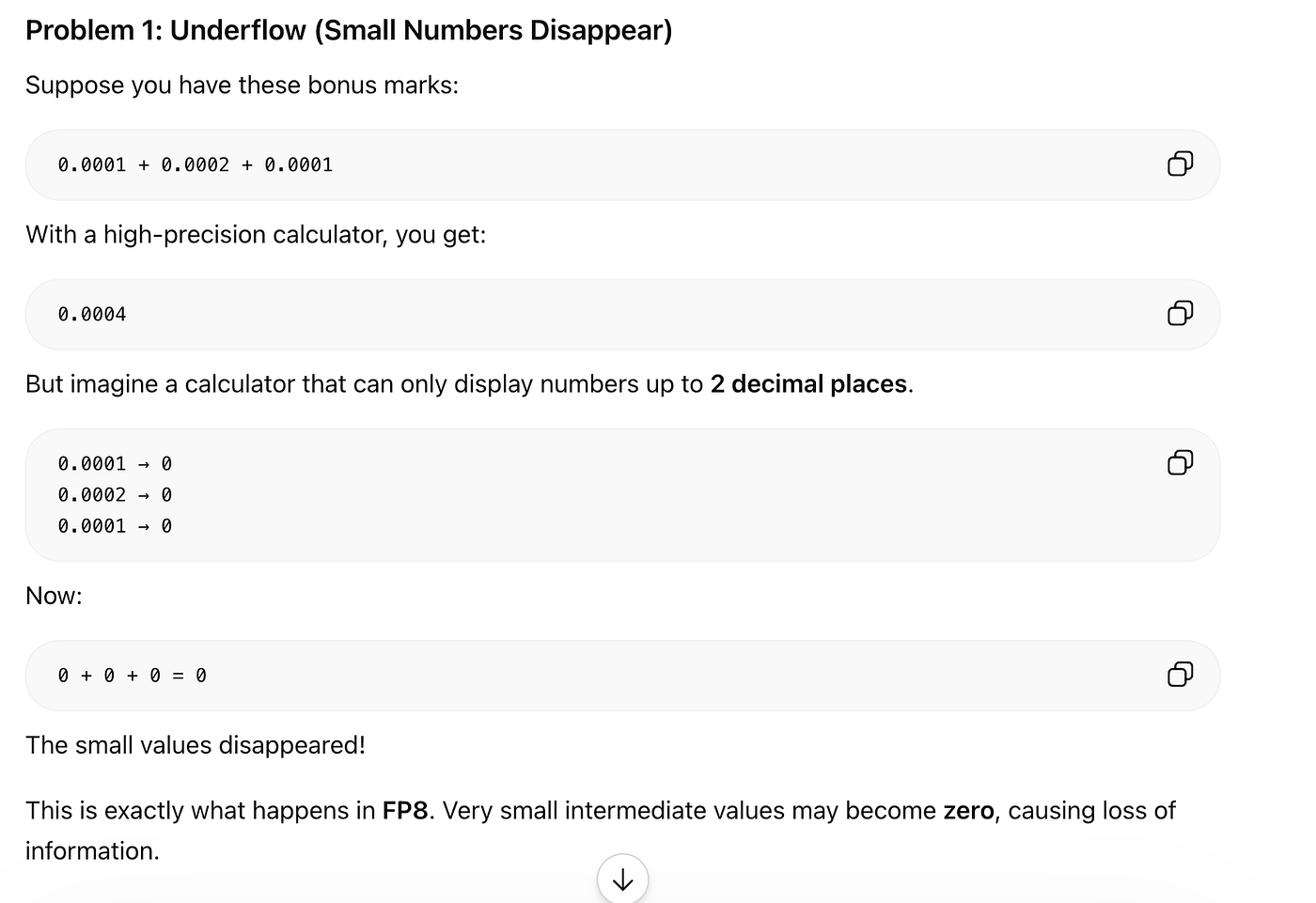
Underflow

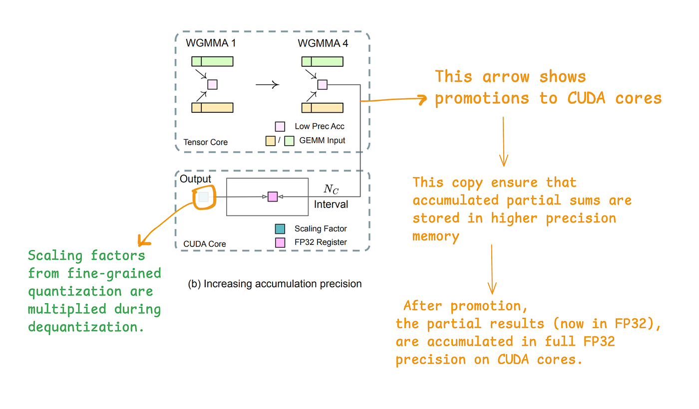
Limited accumulation precision: NVIDIA Tensor Cores (such as on the H800 GPU) accumulate GEMM results internally with limited precision (~14 bits), far below standard FP32 accumulation precision.

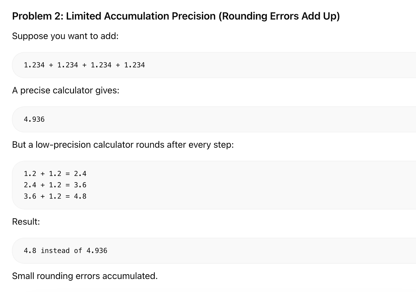
Limited Accumulation Precision

When performing GEMM (General Matrix Multiplication) operations with large inner dimensions K, low accumulation precision can cause errors to accumulate over many additions, leading to significant numerical inaccuracies in the final result.

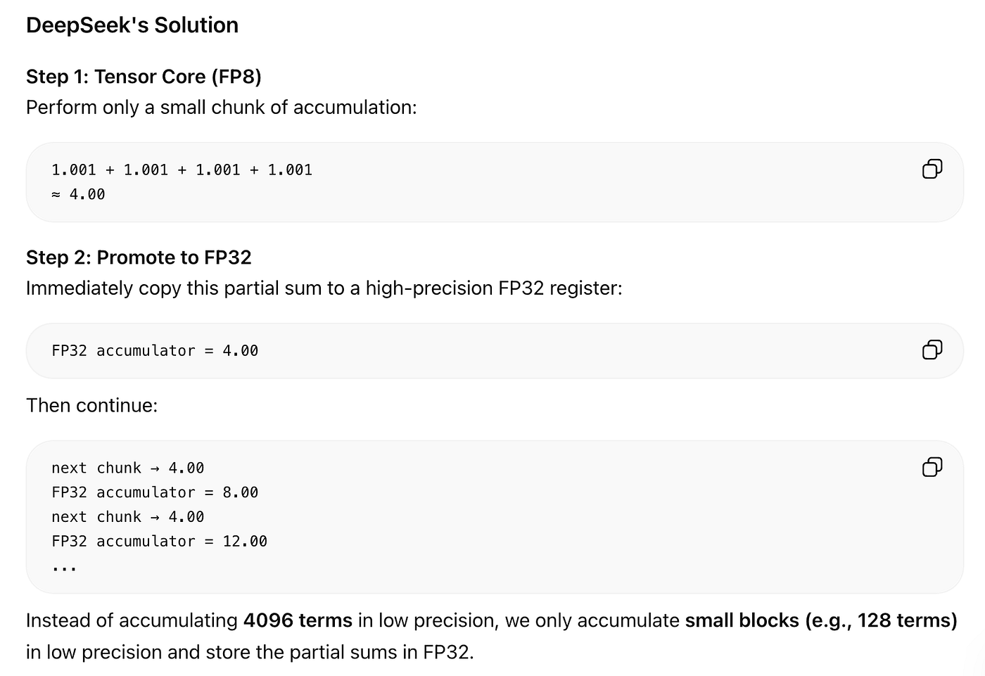
For eg: When multiplying matrices with a large inner dimension (K=4096 ), low accumulation precision can introduce relative errors of up to approximately 2%, significantly degrading model accuracy.

To address this issue, DeepSeek increased the accumulation precision as follows

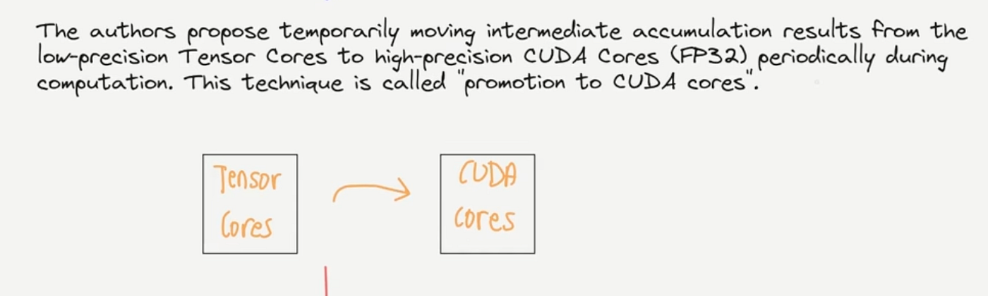
DeepSeek Proposed two step:

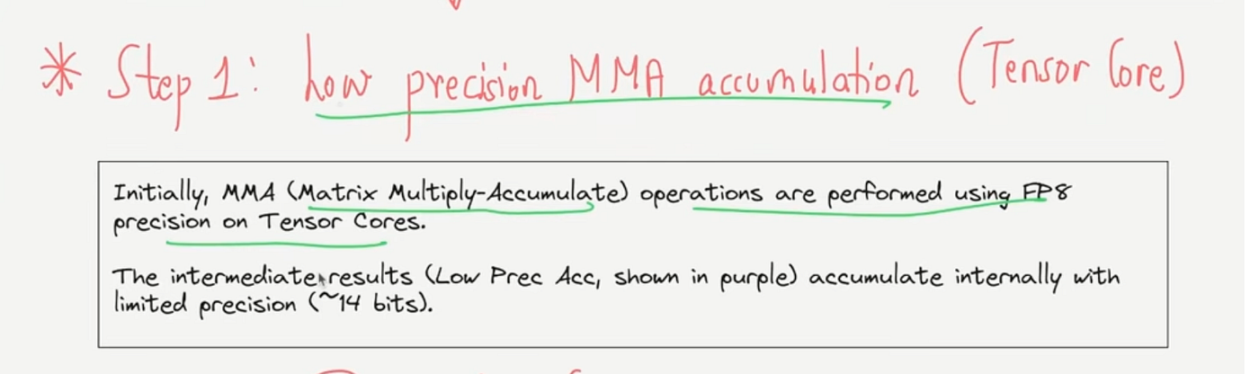
DeepSeek’s Solution

Increasing acummulation precision

4) Mantissa over Exponents

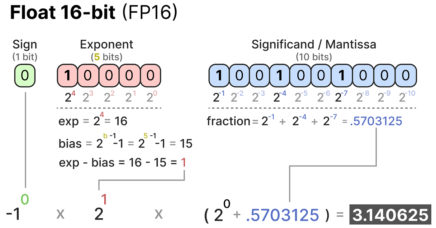
This diagram shows how the number 3.140625 is stored in the FP16 (16-bit floating-point) format.

FP16 uses 1 sign bit, 5 exponent bits, and 10 mantissa (fraction) bits.

The sign bit determines whether the number is positive or negative, the exponent controls the scale or range of the number, and the mantissa stores the precise fractional part.

Together, these three components reconstruct the original value.

In general, more exponent bits increase the range of representable numbers, while more mantissa bits improve numerical precision.

In FP-8, the number of bits allocated for mantissa (precision) and exponent (dynamic range) heavily influence numerical precision and representable range.

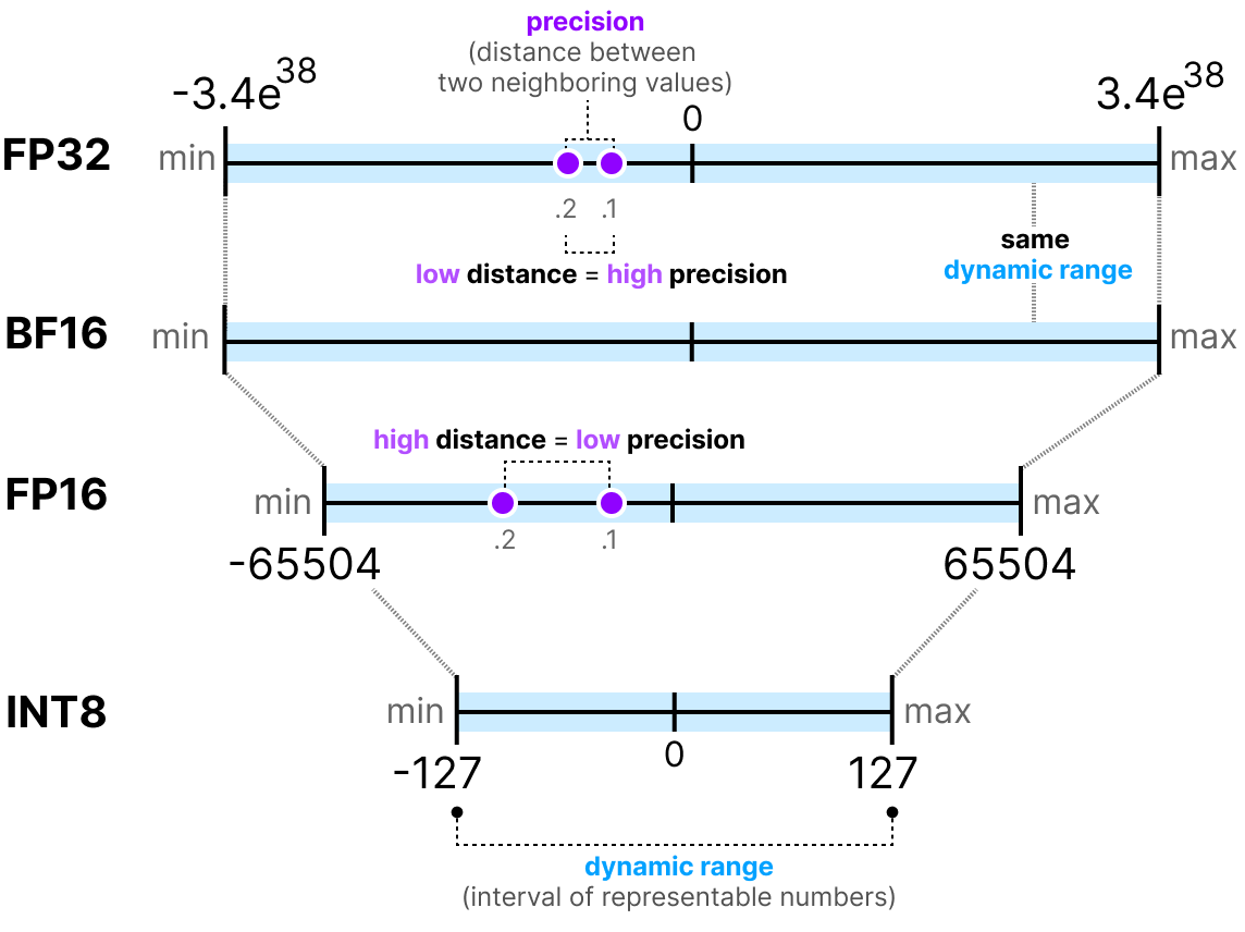
Dynamic range is the range between the smallest and largest values a number format can represent.

From the diagram:

• FP32 & BF16 → very large dynamic range.
• FP16 → smaller dynamic range.
• INT8 → smallest dynamic range.

Larger dynamic range = fewer overflow and underflow problems.

E4M3 vs E5M2

E5M2 (5 exponent bits, 2 mantissa bits):

1. Larger numerical range but lower precision.
2. Good for avoiding overflow/underflow (numbers too large or too small).

E4M3 (4 exponent bits, 3 mantissa bits):

1. Smaller numerical range but higher precision.
2. Good for accurate representation of numbers, but more prone to overflow/underflow issues.

E4M3 vs E5M2 in FP8 Training

Earlier FP8 training approaches typically used different FP8 formats for different stages of training. The forward pass used E4M3, which provides higher precision due to its larger mantissa, while the backward pass (Dgrad and Wgrad computations) used E5M2, which offers a wider numerical range and helps reduce overflow and underflow issues during gradient calculations.

DeepSeek adopted a different strategy. Instead of switching between FP8 formats, it uses E4M3 uniformly for both forward and backward passes. This is possible because DeepSeek employs fine-grained quantization, which applies scaling factors to smaller blocks of data. As a result, numerical values remain well-scaled, allowing E4M3’s higher precision to be used throughout training without suffering from significant overflow or underflow problems.

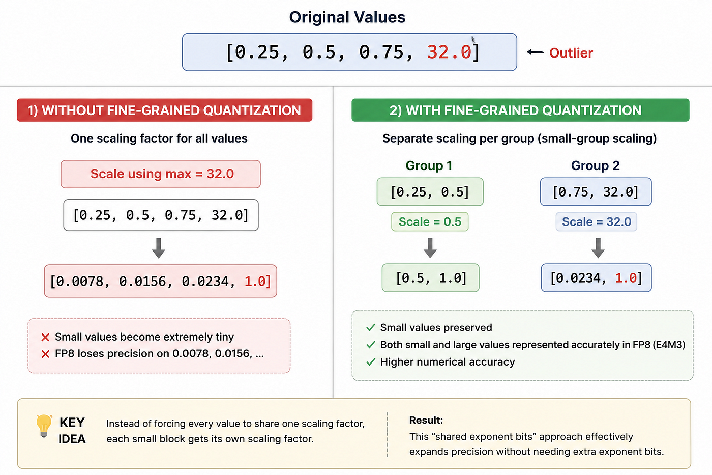
Fine-Grained Quantization

Without fine-grained quantization, a large outlier value (32.0) forces all values to share the same scale, causing small values like 0.25 and 0.5 to shrink to 0.0078 and 0.0156, where FP8 loses precision.

Fine-grained quantization solves this by splitting values into small groups and assigning a separate scaling factor to each group.

This allows both small and large values to be represented accurately in FP8 E4M3, effectively increasing precision without adding extra bits.

5) Online Quantization

Delayed Quantization (Previous Method)

1. The scale factor used for quantizing the current tensor is derived from historical information (e.g., maximum absolute values from past iterations).
2. This means you’re using the past maximum to scale the current tensor, which can be inaccurate if the data distribution changes rapidly.

Main Issue

If the current tensor has a significantly different range, it can lead to overflow or underflow.

DeepSeek’s Solution: Online Quantization

Online Quantization calculates the scale factor in real-time (at each forward/backward pass), based only on the current tensor’s data.

In this method:

• For each small group of elements (activation tile of size 1×128 or weight block of size 128×128), the maximum absolute value is computed on-the-fly.
• This maximum absolute value is immediately used to compute a scaling factor.
• The tensor is then immediately quantized into FP8 using this freshly calculated scaling factor.

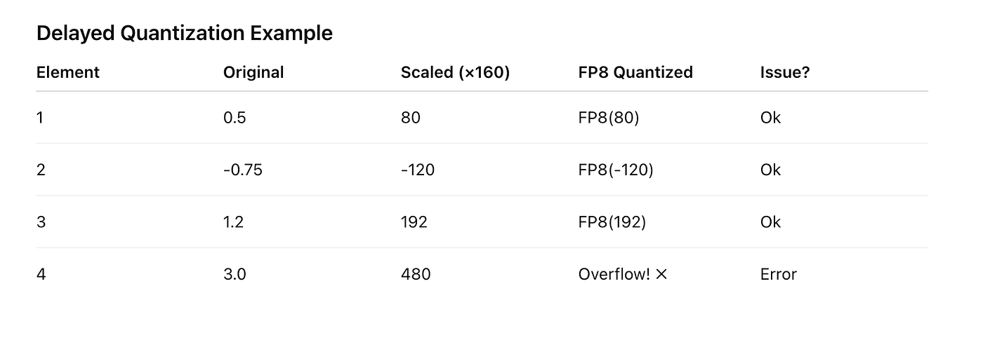
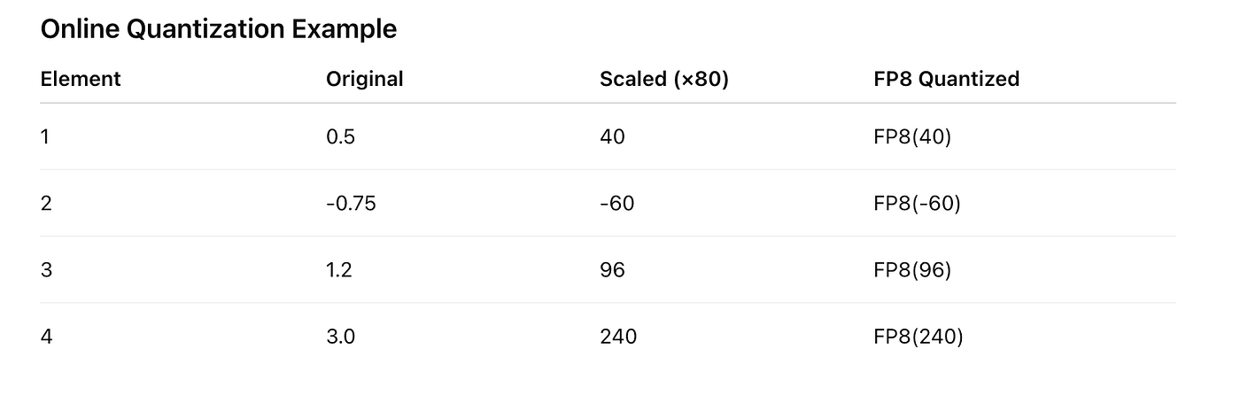
Delayed and Online Quantization Example

Delayed quantization uses scaling factors from previous tensors and may cause overflow/underflow when data distributions change, whereas DeepSeek’s online quantization computes scaling factors from the current tensor in real time, ensuring more accurate and stable FP8 quantization.