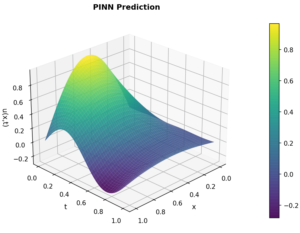
Solving the Heat Equation with Physics-Informed Neural Networks: PyTorch vs TensorFlow

Reference: This article builds on my previous work: Solving the Heat Equation with Physics-Informed Neural Networks: A Practical Guide found here. For a detailed introduction to the core PINN concepts and the PDE problem definition, please refer to that article.

Introduction

In the previous article, we built a PINN from scratch using TensorFlow to solve a 1D heat equation with a source term. The network learned to satisfy the PDE without any labeled solution data, purely by embedding the physical laws into its loss function.

While the TensorFlow implementation was successful, there is growing interest in the PyTorch ecosystem for scientific computing, particularly for research and rapid prototyping. In this article, we’ll:

1. Convert the entire PINN workflow to PyTorch
2. Explain the key differences between the TensorFlow and PyTorch implementations
3. Compare the performance and accuracy of both frameworks side-by-side
4. Provide a complete, reusable PyTorch PINN template

1. PyTorch PINNs Implementation

The full code is available on GitHub. Let’s break down the key components.

1.1 Problem Definition (Identical to TensorFlow)

The problem remains unchanged. We consider the 1D heat equation with a source term, same initial and boundary conditions and of course same exact solution.

1.2 Generating Training Data (Same Strategy)

We use 3,000 random interior collocation points, 150 initial condition points at t=0, and 20 boundary points per edge (mix of grid and random points).

def generate_training_data(n_interior=3000, n_ic=150, n_bc=20, n_bc_grid=5, seed=42):
    np.random.seed(seed)
    X_interior = np.random.rand(n_interior, 2).astype(np.float32)
    # ... (identical to TensorFlow version)
    return X_interior, X_ic, y_ic, X_bc, y_bc

1.3 Neural Network Architecture (Same Structure)

The network has 3 hidden layers with 64 neurons each and tanh activation:

class PINN(nn.Module):
    def __init__(self, hidden_layers=3, hidden_units=64):
        super(PINN, self).__init__()
        layers = []
        layers.append(nn.Linear(2, hidden_units))
        layers.append(nn.Tanh())
        for _ in range(hidden_layers - 1):
            layers.append(nn.Linear(hidden_units, hidden_units))
            layers.append(nn.Tanh())
        layers.append(nn.Linear(hidden_units, 1))
        self.net = nn.Sequential(*layers)

        # Xavier (Glorot) uniform initialization
        def init_weights(m):
            if isinstance(m, nn.Linear):
                nn.init.xavier_uniform_(m.weight)
                nn.init.zeros_(m.bias)
        self.apply(init_weights)

    def forward(self, x):
        return self.net(x)

Note: The explicit class definition is PyTorch’s idiomatic way, equivalent to TensorFlow’s Sequential API.

1.4 The Heart of PINNs: Computing PDE Residuals with torch.autograd

This is where the most significant difference lies. In TensorFlow, we used tf.GradientTape(persistent=True) to compute first and second derivatives:

with tf.GradientTape(persistent=True) as tape:
    u = model(tf.concat([x, t], axis=1))
    u_x = tape.gradient(u, x)
    u_xx = tape.gradient(u_x, x)
    u_t = tape.gradient(u, t)

In PyTorch, we use torch.autograd.grad() in a similar but slightly more explicit manner:

# Forward pass
u = model(torch.cat([x_int, t_int], dim=1))

# Compute derivatives
u_x = torch.autograd.grad(u, x_int, grad_outputs=torch.ones_like(u), create_graph=True)[0]
u_xx = torch.autograd.grad(u_x, x_int, grad_outputs=torch.ones_like(u_x), create_graph=True)[0]
u_t = torch.autograd.grad(u, t_int, grad_outputs=torch.ones_like(u), create_graph=True)[0]

The key points are:

• grad_outputs=torch.ones_like(u) provides the initial gradient vector
• create_graph=True enables second-order differentiation (essential for PINNs)
• We access the first element of the returned tuple (the actual gradient)

1.5 Training Loop

The training loop follows the same structure as TensorFlow:

def train_pinn(model, X_interior, X_ic, y_ic, X_bc, y_bc, ...):
    # Convert data to torch tensors
    X_int_t = torch.tensor(X_interior, requires_grad=True)
    # ... move to device, define optimizer, etc.

    for epoch in range(epochs):
        optimizer.zero_grad()

        # Compute PDE residual, IC, BC losses
        # ...

        loss_total.backward()
        torch.nn.utils.clip_grad_norm_(model.parameters(), 1.0)
        optimizer.step()
        scheduler.step()

Key differences to note:

• PyTorch uses .zero_grad() explicitly before each backward pass
• Gradient clipping with clip_grad_norm_ instead of tf.clip_by_global_norm
• Explicit device management with .to(device)

2. Key Differences Between TensorFlow and PyTorch for PINNs

| Aspect                    | TensorFlow (tf.keras)                              | PyTorch (nn.Module)                          |
|---------------------------|----------------------------------------------------|----------------------------------------------|
| Model Definition          | Sequential API with layer objects                  | Class inheriting from `nn.Module`            |
| Automatic Differentiation | `tf.GradientTape(persistent=True)`                 | `torch.autograd.grad(..., create_graph=True)`|
| Gradient Application      | `optimizer.apply_gradients(zip(grads, variables))` | `optimizer.step()` after `loss.backward()`   |
| Gradient Zeroing          | Ephemeral tape (discarded each epoch)              | Explicit `optimizer.zero_grad()`             |
| Device Management         | Automatic with `tf.device`                         | Explicit with `.to(device)` and `.cuda()`    |

Note: For second‑order derivatives, PyTorch requires create_graph=True to retain the gradient graph – a small but important detail for PINNs.

3. Results and Visualization

After training for 8000 epochs, we achieve excellent agreement with the exact solution:

PyTorch PINN Results:

• Mean Squared Error (MSE): 2.592 × 10⁻⁵
• L2 Error: 5.115 × 10⁻³
• L∞ Error: 2.381 × 10⁻²

The figures below show the 3D surface comparison, loss curves, and solution snapshots.

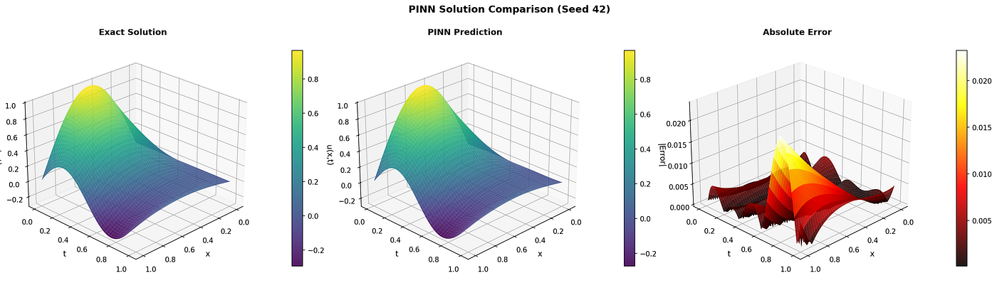
Figure 1: 3D Solution Comparison

Figure 2: Solution Snapshots at Different Times

Figure 3: Loss Curves During Training

4. Point-by-Point Comparison: PyTorch vs. TensorFlow

I ran both implementations on the same hardware (NVIDIA RTX 4050 Laptop GPU) for a fair comparison. The hyperparameters were identical across both runs (8000 epochs, 3×64 architecture, polynomial learning rate schedule).

TensorFlow Environment: tensorflow-gpu 2.10.1, CUDA 11.8, cuDNN 8.1 PyTorch Environment: torch 2.5.1+cu118, CUDA 11.8

| Metric                    | TensorFlow      | PyTorch          | Winner          
|---------------------------|-----------------|------------------|-----------------
| Final L2 Error            | 3.649 × 10⁻³    | 5.115 × 10⁻³     | TF (30% lower)  
| Final MSE                 | 1.319 × 10⁻⁵    | 2.592 × 10⁻⁵     | TF              
| L∞ Error                  | 1.814 × 10⁻²    | 2.381 × 10⁻²     | TF              
| Training Time (8000 ep.)  | 333.6 sec       | 119.6 sec        | PT (2.8× faster)

Analysis:

• Accuracy: TensorFlow achieves approximately 30% lower L2 error, suggesting its optimization path and automatic differentiation may be slightly better suited for this particular PDE.
• Speed: PyTorch trains nearly three times faster, making it more efficient for rapid experimentation and iterative development.

5. Why These Differences Occur

Several factors explain the observed differences:

1. Numerical Precision: By default, PyTorch disables TF32 for matrix multiplications, while TensorFlow may handle this differently depending on the version. Since these settings were not explicitly aligned, the two frameworks may have operated at slightly different numerical precisions, which could partially explain the observed accuracy gap.
2. Automatic Differentiation Implementation: TensorFlow’s GradientTape and PyTorch's autograd.grad use different graph construction strategies. While both produce correct results, subtle differences in how second derivatives are cached and reused can affect both speed and numerical stability.
3. Framework Maturity for PINNs: PINNs require second-order automatic differentiation, which both frameworks handle well. TensorFlow was used in the seminal PINN papers by Raissi et al. (2019), giving it historical precedence. However, modern PINN libraries (e.g., DeepXDE) support both frameworks, and the current landscape is largely framework‑agnostic.

Note: Even with identical seeds, the initial weight values differ because the random number generators are not synchronised across frameworks. This is unavoidable and does not bias the comparison — the statistical distribution (Xavier uniform) is the same.

6. Conclusion and Recommendations

For Research and Prototyping: PyTorch’s speed (2.8× faster) and Pythonic design make it ideal for rapid iteration and experimentation. The code is intuitive and easier to debug, which is valuable when trying new network architectures or loss formulations.

For Production and Highest Accuracy: TensorFlow’s slightly better final accuracy may be preferred for applications where every bit of precision matters, such as scientific simulations or engineering design. (Note: this conclusion is based on a single run; multiple random seeds would be needed to confirm statistical significance.)

What I Learned:

• Both frameworks are fully capable of implementing PINNs
• The choice should be driven by your specific priorities (accuracy vs. speed)
• Framework differences are smaller than often assumed — the same architecture and hyperparameters yield comparable results

The complete PyTorch implementation is available on GitHub. Feel free to adapt it for your own PDEs and experiments.

Tags: #MachineLearning #ScientificMachineLearning #PhysicsInformedNeuralNetworks #PINNs #ScientificComputing #DeepLearning #HeatEquation #PyTorch #TensorFlow