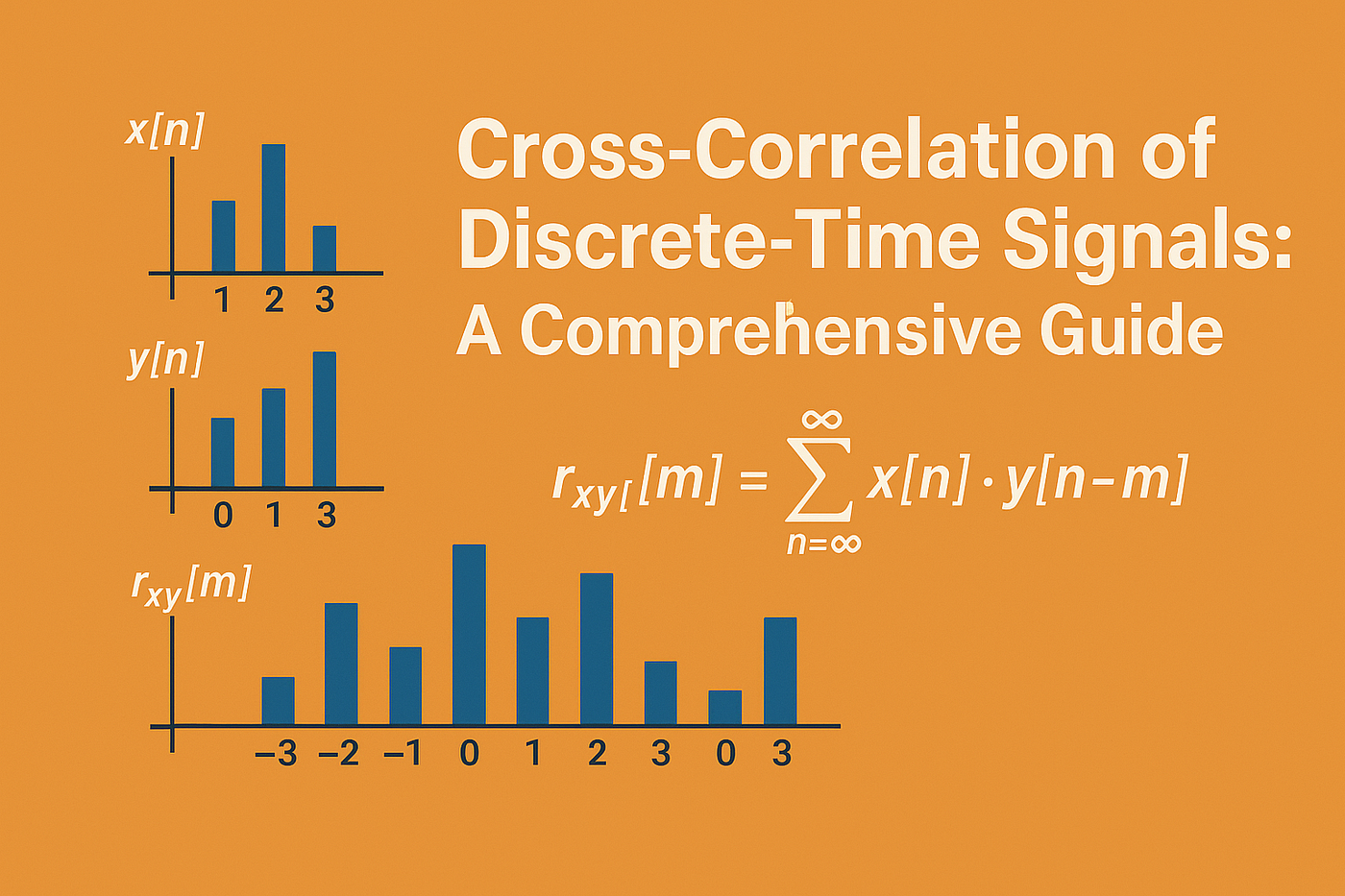
Cross-Correlation of Discrete-Time Signals: A Comprehensive Guide

Signal processing forms the backbone of modern communication systems, control systems, and various data analysis techniques. Among the fundamental operations in discrete-time signal processing, cross-correlation stands out as a powerful tool for comparing the similarity between two signals. This blog post delves into the concept of cross-correlation, its mathematical formulation, computational methods, and practical applications through a detailed example.

Introduction

Cross-correlation is a measure of similarity between two signals as a function of the displacement of one relative to the other. It is particularly useful in pattern recognition, signal detection, and feature extraction. Unlike autocorrelation (which compares a signal with itself), cross-correlation compares two different signals and provides insights into how they relate to each other at different time shifts.

In many practical applications — ranging from radar and sonar systems to speech recognition and image processing — cross-correlation helps in identifying patterns, detecting signals amidst noise, and extracting meaningful information from complex data.

Mathematical Foundation

Definition

For two discrete-time signals x[n] and y[n], the cross-correlation sequence rxy[m] is defined as:

rxy​[m]=∑n=−∞∞​x[n]⋅y[n−m]

Where:

• x[n] is the first signal
• y[n] is the second signal
• m represents the time shift (lag) between the signals
• rxy[m] is the cross-correlation value at lag m

The formula essentially slides one signal (y[n]) past the other (x[n]) and computes the sum of their products at each position.

Properties of Cross-Correlation

1. Non-commutative: Unlike convolution, cross-correlation is not commutative. That is, rxy[m] ≠ ryx[m] in general.
2. Time reversal relation: The cross-correlation of x[n] and y[n] equals the convolution of x[n] and y[-n]:

rxy​[m]=x[n].y[−n]

3. Energy relationship: If the signals are energy signals, the maximum value of the cross-correlation is bounded by the geometric mean of their energies:

4. Relation to the frequency domain: The cross-correlation theorem states that the Fourier transform of the cross-correlation equals the product of the Fourier transform of one signal and the complex conjugate of the Fourier transform of the other:

Computational Methods

There are several ways to compute the cross-correlation between two signals:

1. Direct Method

The direct method involves applying the definition formula directly:

For finite-length sequences of lengths N₁ and N₂, the range of m and the summation limits need to be adjusted. The length of the cross-correlation sequence is N₁ + N₂ — 1.

2. Matrix Method

The matrix method organizes the computation in a tabular format, making it easier to track the multiplications and additions:

1. Arrange one signal along rows and the other along columns
2. Multiply the corresponding elements
3. Sum the products for each lag m

3. Tabular Method

The tabular method provides a systematic way to align the signals for different lags and compute the products:

1. Create a table with rows representing different lags
2. Align the signals according to each lag
3. Compute the products and sum them for each lag

4. Frequency Domain Method

Using the Fast Fourier Transform (FFT), cross-correlation can be computed more efficiently:

1. Compute the FFT of both signals
2. Multiply the FFT of the first signal with the complex conjugate of the FFT of the second signal
3. Compute the inverse FFT of the product

Practical Example: Cross-Correlation Calculation

Let’s work through a detailed example to illustrate how cross-correlation is computed in practice.

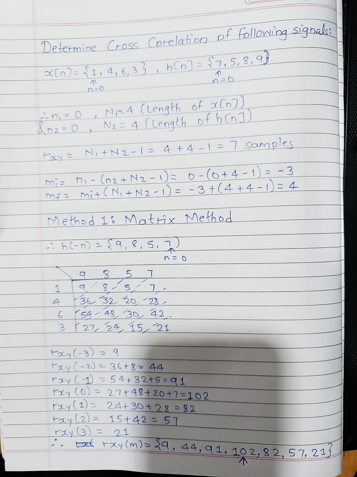
Given two discrete-time signals:

• x[n] = {1, 4, 6, 3} for n = 0, 1, 2, 3 respectively
• y[n] = {7, 5, 8, 9} for n = 0, 1, 2, 3 respectively

We want to determine the cross-correlation sequence rxy[m].

Step 1: Determine the Range of m

For signals of lengths N₁ = 4 and N₂ = 4, the cross-correlation will have N₁ + N₂ — 1 = 7 values.

The range for m will be from -(N₂-1) to (N₁-1), which is from -3 to 3.

Step 2: Calculate Initial Parameters

• n₁ = 0 (starting index of x[n])
• N₁ = 4 (length of x[n])
• n₂ = 0 (starting index of y[n])
• N₂ = 4 (length of y[n])
• Lxy = N₁ + N₂ — 1 = 4 + 4–1 = 7 samples
• m₁ = n₁ — (n₂ + N₂ — 1) = 0 — (0 + 4–1) = -3
• m₂ = m₁ + (N₁ + N₂ — 1) = -3 + (4 + 4–1) = 4

Method 1: Matrix Method

To implement the matrix method, we create a table where we multiply each element of x[n] with each element of y[n]:

y[0]=7  y[1]=5  y[2]=8  y[3]=9
x[0]=1   7      5      8      9
x[1]=4   28     20     32     36
x[2]=6   42     30     48     54
x[3]=3   21     15     24     27

Now, we compute rxy[m] for each value of m:

• rxy[-3] = 9 (single element at the bottom-right diagonal)
• rxy[-2] = 36 + 8 = 44 (sum of elements on the next diagonal)
• rxy[-1] = 54 + 32 + 5 = 91 (sum of elements on the next diagonal)
• rxy[0] = 27 + 48 + 20 + 7 = 102 (sum of elements on the main diagonal)
• rxy[1] = 24 + 30 + 28 = 82 (sum of elements on the next diagonal)
• rxy[2] = 15 + 42 = 57 (sum of elements on the next diagonal)
• rxy[3] = 21 (single element at the top-left diagonal)

Therefore, rxy[m] = {9, 44, 91, 102, 82, 57, 21} for m = -3, -2, -1, 0, 1, 2, 3 respectively.

Method 2: Tabular Method

The tabular method provides another perspective by explicitly showing how the signals align at each lag:

n      -3  -2  -1   0   1   2   3   4   5   6
x[n]                1   4   6   3
y[n]                7   5   8   9

For m = -3, y[n-(-3)] = y[n+3]:

n      -3  -2  -1   0   1   2   3   4   5   6
x[n]                1   4   6   3
y[n+3]   7  5   8   9

rxy[-3] = 1×9 = 9

For m = -2, y[n-(-2)] = y[n+2]:

n      -3  -2  -1   0   1   2   3   4   5   6
x[n]                1   4   6   3
y[n+2]       7  5   8   9

rxy[-2] = 1×8 + 4×9 = 8 + 36 = 44

For m = -1, y[n-(-1)] = y[n+1]:

n      -3  -2  -1   0   1   2   3   4   5   6
x[n]                1   4   6   3
y[n+1]           7  5   8   9

rxy[-1] = 1×5 + 4×8 + 6×9 = 5 + 32 + 54 = 91

For m = 0, y[n-0] = y[n]:

n      -3  -2  -1   0   1   2   3   4   5   6
x[n]                1   4   6   3
y[n]                7   5   8   9

rxy[0] = 1×7 + 4×5 + 6×8 + 3×9 = 7 + 20 + 48 + 27 = 102

For m = 1, y[n-1]:

n      -3  -2  -1   0   1   2   3   4   5   6
x[n]                1   4   6   3
y[n-1]                  7   5   8   9

rxy[1] = 4×7 + 6×5 + 3×8 = 28 + 30 + 24 = 82

For m = 2, y[n-2]:

n      -3  -2  -1   0   1   2   3   4   5   6
x[n]                1   4   6   3
y[n-2]                      7   5   8   9

rxy[2] = 6×7 + 3×5 = 42 + 15 = 57

For m = 3, y[n-3]:

n      -3  -2  -1   0   1   2   3   4   5   6
x[n]                1   4   6   3
y[n-3]                          7   5   8   9

rxy[3] = 3×7 = 21

Therefore, using the tabular method, we confirm: rxy[m] = {9, 44, 91, 102, 82, 57, 21} for m = -3, -2, -1, 0, 1, 2, 3 respectively.

Interpretation of Results

The cross-correlation sequence rxy[m] provides information about the similarity between signals x[n] and y[n] at different time shifts. Several observations can be made from our example:

1. Maximum value: The cross-correlation reaches its maximum value of 102 at m = 0, indicating that the signals have the highest similarity when they are aligned without any shift.
2. Symmetry: The cross-correlation sequence isn’t perfectly symmetric, which is expected since cross-correlation is generally not symmetric unless the signals themselves have special properties.
3. Decay pattern: The values decrease as we move away from the peak in either direction, suggesting that the similarity between the signals diminishes with increasing time shift.

Applications of Cross-Correlation

Cross-correlation finds applications in numerous fields:

1. Signal Detection: In radar and sonar systems, cross-correlation helps detect the presence of known signals amidst noise.
2. Pattern Recognition: In image processing, cross-correlation can locate templates within larger images.
3. Time Delay Estimation: By finding the lag where cross-correlation peaks, we can estimate the time delay between two similar signals.
4. Speech Processing: Cross-correlation aids in voice activity detection and speaker recognition.
5. Biomedical Signal Analysis: It helps analyze EEG, ECG, and other biological signals.
6. Communication Systems: Cross-correlation is used in spread spectrum systems for synchronization and code acquisition.

Conclusion

Cross-correlation is a fundamental operation in discrete-time signal processing that quantifies the similarity between two signals as a function of time shift. Through the mathematical formulation and the practical example we explored, it’s evident that cross-correlation provides valuable insights into signal relationships.

The methods discussed — direct calculation, matrix method, tabular method, and frequency domain approach — offer different perspectives and computational efficiencies for determining cross-correlation. Depending on the specific application and computational resources available, one method might be more suitable than others.

As signal processing continues to evolve and find applications in emerging fields like artificial intelligence and IoT, understanding operations like cross-correlation becomes increasingly important. Whether you’re a student, researcher, or industry professional, mastering cross-correlation equips you with a powerful tool for analyzing and extracting meaningful information from discrete-time signals.

References

1. Oppenheim, A. V., & Schafer, R. W. (2010). Discrete-Time Signal Processing (3rd ed.). Pearson.
2. Proakis, J. G., & Manolakis, D. G. (2006). Digital Signal Processing (4th ed.). Pearson.
3. Hayes, M. H. (1996). Statistical Digital Signal Processing and Modeling. Wiley.
4. Smith, S. W. (1997). The Scientist and Engineer’s Guide to Digital Signal Processing. California Technical Publishing.