Linear and Logistic Regression

If you’ve spent any time in the realm of machine learning, you’ve probably heard linear regression and logistic regression, often described as “beginner” models — the models you learn first and then move past.

That framing never quite sat right with me.

Yes, you can pick these up early. But these same models show up in production forecasting systems, clinical research, financial risk models, and A/B testing pipelines at some of the most sophisticated organizations in the world. To me, “beginner” doesn’t mean “limited”; it means “foundational.”

And that’s exactly what makes them worth understanding deeply. Buried inside these two models are the core ideas that power almost every concept in machine learning:

• How models learn from data
• How predictions are made
• How loss functions work
• How optimization works
• How coefficients can be interpreted
• How probability enters machine learning

Think of this post as a proper introduction, one that doesn’t just show you the equations and how they work, but also explains the intuition behind them, the assumptions you’re making, how to evaluate your results, and where things can go wrong.

The Big Picture

At a high level, both models aim to learn a relationship between inputs and outputs.

We usually write the input features as:

and the target variable (i.e., output) as:

The difference is in the type of target we want to predict.

Linear Regressions predict a continuous value (e.g., house price, salary, temperature). Logistic regression predicts a class probability (e.g., spam or not spam, churn or not churn).

A simple mental model:

Part 1: Linear Regression

What Is Linear Regression?

Linear regression models the relationship between one or more input variables and a continuous output variable.

The simplest version of a linear regression uses one feature to predict one target.

For example:

Can we predict someone’s annual income based on years of experience?

The model assumes the relationship can be approximated by a straight line.

If this looks familiar, it should. This is exactly the y = mx + b equation from your first algebra class, just written with different letters. β₀ is the slope (your old m), and β₁ is the intercept (your old b). Linear regression is, at its core, fitting a line. The difference is that instead of drawing it by hand, we’re letting the model find the line that best fits real data.

Where:

• ŷ is the predicted value
• x is the input feature
• β₀ is the slope
• β₁ is the intercept

The intercept tells us the predicted value when x = 0.

If x is your only feature, the slope tells us how much ŷ changes when x increases by one unit.

When you have more than one feature, the equation extends naturally; this is called multiple linear regression:

For example, to predict house price using size, number of bedrooms, and age:

Each coefficient (βᵢ) measures the effect of one feature while holding the others constant. Same idea as the single-feature case, just more variables on the line.

A Simple Linear Regression Diagram

Imagine we have data points showing house size and house price. Linear regression fits the best straight line through those points.

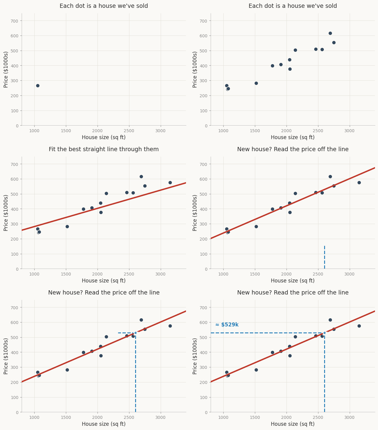
That line becomes our prediction rule. Given a new house size, we can plug it into the equation and estimate the price.

Visualizing Residuals

Before we can talk about what “best fit” means, we need to understand one key concept: a residual.

A residual is the difference between what actually happened and what the model predicted.

Where:

• eᵢ is the residual
• yᵢ is the actual value
• ŷᵢ is the predicted value

In the diagram below, each vertical gap between a data point and the regression line is a residual. If a point is above the line, the residual is positive. If a point is below the line, the residual is negative. The larger the gap, the worse the prediction for that observation.

What Does “Best Fit” Mean?

Now “best fit” has a more precise meaning: linear regression tries to find the line that makes those residuals collectively as small as possible.

Real-world data is noisy, so we usually cannot draw a line that hits every point perfectly. The model needs a rule for deciding which imperfect line is best.

The most common rule is to minimize the sum of squared residuals:

Or the mean squared error:

Squaring the residuals does two useful things: it prevents positive and negative errors from canceling each other out, and it penalizes big mistakes more heavily than small ones.

MSE is a sensible default, but it’s not your only option. Because squaring errors makes big mistakes count disproportionately, MSE is useful when you really want to avoid big misses, but less ideal if your data has outliers you don’t want the model chasing. In those cases, Mean Absolute Error (MAE) is often a better fit since it treats all errors equally regardless of size. There are many other loss functions too; Huber loss, for example, blends the two by behaving like MSE for small errors and MAE for large ones. The right choice depends on how much you care about outliers and what kinds of errors are most costly for your problem.

The Closed-Form Solution

One reason linear regression is mathematically elegant is that the basic version has a closed-form solution (an exact answer obtained directly from a finite formula, rather than arriving at it through repeated approximations like gradient descent).

The optimal coefficient vector is:

This is called the ordinary least squares solution.

However, in large-scale machine learning, we often use iterative optimization methods such as gradient descent, especially when:

• The dataset is very large
• There are many features
• We use regularization
• Matrix inversion is computationally expensive

Gradient Descent for Linear Regression

Gradient descent updates coefficients step by step to reduce the loss.

The cost function J(β) measures how wrong the model currently is; it’s the average squared error across all training examples (we place 1/(2n) outside the sum because it is a constant, so we can, and it makes the derivative cleaner):

The update rule says: take each coefficient, figure out which direction would reduce the cost, and nudge it a small step in that direction. α (the learning rate) controls how big each step is; too large, and you may overshoot the minimum; too small, and convergence may take much longer:

Where:

• α is the learning rate
• ∂J/∂βⱼ is the gradient
• j indexes a coefficient

The gradient ∂J/∂βⱼ tells us the slope of the cost function with respect to each coefficient. For linear regression, it works out to the average of each prediction error (yᵢ − ŷᵢ) weighted by the corresponding feature value xᵢⱼ; intuitively, features that contributed more to the error get a bigger correction:

The intuition:

Move the coefficients in the direction that reduces prediction error.

Interpreting Linear Regression Coefficients

Suppose we fit this model:

Then:

• The intercept is 50000.
• Each additional square foot increases predicted price by 200, holding bedrooms constant.
• Each additional bedroom increases predicted price by 15000, holding size constant.

This “holding all else constant” interpretation is one of linear regression’s biggest strengths.

It is not just predictive. It is interpretable.

Key Assumptions of Linear Regression

Linear regression doesn’t require perfect data, but it does have a few expectations. Violating them doesn’t always break your model, but it’s worth knowing when you’re on shaky ground.

1. Linearity

The relationship between your features and target should be roughly linear. If the true pattern is a curve, the model will struggle to capture it. A good way to test this before trying this model is to visualize the data with a scatterplot.

2. Independent Errors

The errors shouldn’t be correlated with each other. (e.g., students from the same school or patients from the same hospital).

3. Constant Variance

The spread of your errors should stay roughly the same across all predicted values; this is called homoscedasticity. A healthy residual plot looks like random noise scattered evenly around zero. A problematic one fans out, with errors growing larger as predictions increase. If you see that fanning pattern, it’s a sign your model is less reliable at the high end of its range.

4. No Severe Multicollinearity

If two features are highly correlated, the model has a hard time figuring out which one is doing the work. Coefficients become unstable and lose their interpretability.

Evaluating Linear Regression

The most common metrics are MAE, MSE, RMSE, and R². MAE gives you the average error in plain units, making it easier to interpret. The MSE squares the errors, penalizing large errors more heavily. RMSE brings MSE back to interpretable units. R² tells you how well a model explains the variance in the target variable.

Each of these deserves its own deep dive, but the key thing to know here is: don’t rely on a single metric, and always evaluate on held-out data. A model that looks great on training data can still fall apart in the real world.

Part 2: Logistic Regression

What Is Logistic Regression?

Despite the second part of its name, logistic regression is usually used for classification.

The most common version is binary logistic regression, where the target has two possible classes:

Examples:

• Customer churn: yes or no
• Email spam: spam or not spam
• Loan default: default or no default
• Disease diagnosis: positive or negative

There are extensions for other cases too: multinomial logistic regression handles targets with more than two unordered classes (e.g., predicting whether a user will buy, browse, or leave), and ordinal logistic regression handles ordered categories (e.g., ratings from 1 to 5). But binary is by far the most common, and the core ideas carry over directly, so let’s focus on that for now.

Instead of predicting a continuous value directly, logistic regression predicts a probability.

For example:

“This customer has a 78% probability of churning.”

Why Not Use Linear Regression for Classification?

Suppose we try to use linear regression for a binary target.

The problem is that linear regression can output any number:

But probabilities must be between 0 and 1 (which is a percentage when scaled up to 0–100):

So logistic regression wraps the linear model inside a function that squashes values into the interval (0, 1). That function is the sigmoid function.

The Sigmoid Function

The sigmoid function is:

It maps any real number to a value between 0 and 1.

• When z is very negative, the sigmoid is close to 0.
• When z is 0, the sigmoid is 0.5.
• When z is very positive, the sigmoid function approaches 1.

Logistic Regression Equation

First, logistic regression builds a linear score:

Then it converts that score into a probability:

So the full model is:

The final prediction is often made using a threshold:

The threshold does not have to be 0.5. In medical diagnosis, fraud detection, or safety-critical systems, we may choose a different threshold depending on the cost of false positives and false negatives.

Logistic Regression Loss Function

Linear regression uses squared error as a loss function. Whereas logistic regression uses log loss, also called binary cross-entropy. This is an extremely popular loss function used in some of the most complex models today, so it’s best to make sure you fully understand and remember it.

For one observation:

For the full dataset:

This loss function heavily penalizes confident wrong predictions.

• If the true label is 1 and the model predicts 0.99, the loss is small.
• If the true label is 1 and the model predicts 0.01, the loss is huge.

Gradient Descent for Logistic Regression

Contrary to Linear Regression, Logistic Regression does not have a closed-form solution, so we usually use gradient descent. We derive the gradient below.

Let:

Then the gradient of the average loss is:

The update rule is:

This looks similar to linear regression. The model predicts, compares the prediction to reality, and updates coefficients to reduce error.

Evaluating Logistic Regression

Classification needs different metrics than regression. Accuracy is the obvious starting point: what fraction of predictions were correct, but it breaks down badly with imbalanced classes. A fraud model that never flags anything can still hit 98% accuracy if fraud is rare.

More useful are precision (of what we flagged, how much was real?), recall (of what was real, how much did we catch?), and F1 (a harmonic mean of the two). Which one matters most depends entirely on the cost of each type of mistake; missing a cancer diagnosis is very different from sending a spam email to the wrong folder.

The ROC curve and its summary statistic AUC give a threshold-independent view of model quality, showing how well the model ranks positives above negatives across all possible cutoffs.

Part 3: Regularization

When a model has too many features or features that are correlated, it can start memorizing the training data rather than learning the underlying pattern. That’s overfitting, and regularization is the standard fix.

The idea is simple: add a penalty to the loss function that discourages coefficients from getting too large. The two most common flavors are Ridge (L2) and Lasso (L1).

Ridge squares the coefficients in the penalty term:

Lasso uses absolute values instead:

Ridge shrinks all coefficients toward zero but rarely eliminates any entirely (good when you believe most features contribute something). Lasso can push coefficients all the way to zero, effectively removing features from the model, essentially automating feature selection (useful when you suspect only a subset of your features actually matter).

Both work equally well with linear and logistic regression; you just apply the same penalty to the cross-entropy loss instead. In practice, λ is a hyperparameter you tune (larger values mean more regularization and simpler models).

Part 4: Practical Workflow

Practical Tips for Linear Regression

Reach for linear regression when your target is a continuous number and interpretability matters; it’s hard to beat when you need to explain why the model made a prediction, not just what it predicted. It’s also a great first model to run before trying anything more complex.

The main things to watch for: outliers can pull the line in ways that hurt overall performance, highly correlated features make coefficients unreliable, and the model will happily extrapolate past your training data with no warning. If the relationship looks curved, you don’t have to abandon linear regression; adding polynomial features like x² keeps you in the linear framework while capturing the curve. And if your target is heavily skewed, modeling log(y) instead often helps significantly.

Practical Tips for Logistic Regression

Logistic regression is the natural starting point for any binary classification problem, especially when you need probabilities rather than just a yes/no answer and when being able to explain the model matters.

A few things worth keeping in mind: imbalanced classes are the most common pitfall; if 95% of your data is one class, accuracy will lie to you. And the default 0.5 threshold is just a starting point, not a rule. The right threshold depends on what’s more costly in your situation: a fraud detection model might set it low to catch more suspicious cases, while a content moderation system might set it high to avoid false positives. Think about the cost of each type of mistake before you decide where to cut.

Final Thoughts

Linear regression and logistic regression are not just beginner models.

They are the conceptual foundation of much of machine learning.

Linear regression teaches us how to model continuous outcomes, minimize squared error, interpret coefficients, and understand residuals.

Logistic regression teaches us how to model probabilities, classify outcomes, use cross-entropy loss, interpret odds, and reason about decision thresholds.

Their simplicity is a feature, not a weakness.

When you need a model that is fast, interpretable, mathematically clean, and surprisingly competitive, linear and logistic regression are often the best place to start.

A quick note: we deliberately moved fast through a lot of topics in this post evaluation metrics, regularization, gradient descent, loss functions, and more. Each of these deserves a proper deep dive of its own. Rest assured, we’ll get to them. :)