[New Trend: “Liquid Time Constants”] Integrated Understanding of LFM2 Explained, Latest Linear Architectures (e.g., Mamba2), and Key Points for High-Speed Implementation of State Space Models

Prelude

The moonlight gently illuminates the long nights, it reminds us that rose red leaves.

How are you doing?

My name is Rikka Botan.

In this article I will discuss LFM2: Liquid Foundation Model *1–15, a language model that excels at fast generation, high downstream performance, and edge‑device deployment.

The piece dives deeper into LFM2’s principles and performance from the perspective of Liquid Time‑Constant Ordinary Differential Equations (LTC‑ODEs) *16 17.

I also provide an overview of recent linear modelling techniques, a walkthrough of Mamba 2 implementation, and a discussion of the model’s novel mechanisms.

I hope this humble write‑up proves useful to you.

If you notice any typos or omissions, please feel free to point them out in the comments.

Rikka Botan’s X (Twitter) account:

https://twitter.com/peony__snow

I’ll be sharing the latest progress and tech insights (and sometimes personal updates). If you’re interested, please consider following.

Target Readers

• Comfortable with at least basic Python programming.
• Have a reasonable understanding of CNNs, RNNs, and Transformers.
• Familiar (even if only vaguely) with state‑space models such as S4 or Mamba.
• Interested in grasping LFM2’s principles and design philosophy.

Table of Contents

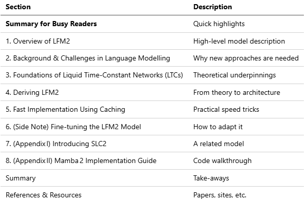
Summary for Busy Readers

• LFM2 combines Gated‑Short Convolution with Grouped Query Attention (GQA).
• It is theoretically grounded in LTCs and can dynamically adapt its behavior to input.
• The model contains a linear‑time‑decaying first‑order system that remains stable even for infinite‑length inputs.
• LFM2 smoothly handles the temporal non‑uniformity that traditional Transformers struggle with.

1. Overview of LFM2

*1

*2–6

LFM2 outperforms the Qwen3 series on CPU by roughly twice the speed while matching its downstream performance.

Its composite structure of Gated‑Short Convolution and Grouped Query Attention.

Liquid AI writes that it is inspired by LTCs.

Because it runs swiftly on CPUs, LFM2 is especially well suited for low‑latency edge applications.

Recently Liquid AI has focused on developing task‑specific models under the Liquid Nanos *7–15 to accelerate edge deployment.

Gated‑Short Conv Block Algorithm

def lfm2_conv(x: Tensor):
B, C, x = linear(x) # input projection
x = B * x # gating (gate depends on input)
x = conv1d(x) # short convolution
x = C * x # gating
x = linear(x)
return x

At first glance this appears to be a simple block, but it is rooted in the LTC‑ODE perspective.

The main goal of this article is to mathematically explain why this implementation excels at modelling discrete sequences.

2. Background and Challenges for Language Models

In domains that process time‑series data or sequential structures — such as natural language processing (NLP), speech, sensor streams, video, etc., autoregressive transformers have demonstrated strong performance on many recent sequence‑modeling tasks thanks to their in‑context learning ability and parallelizable training procedures *18. In particular, SoftMax‑based attention mechanisms capture token dependencies dynamically and have yielded remarkable results during large‑scale pretraining.

However, a fundamental limitation of transformers is that both computational cost and memory usage grow quadratically with sequence length.

*Self‑Attention Formulation 18**

The quadratic cost arises from computing interactions between all token pairs and maintaining large key/value caches. While GPUs can mask this overhead for short sequences, it remains a significant practical bottleneck for long‑form inputs, real‑time inference, or edge deployments.

To address this constraint, recent research has focused on architectures that enable linear‑time, linear‑memory inference. Representative approaches include linear‑attention models 19–25, state‑space models (SSMs) 26–35, neural memory mechanisms 36–39, and top‑k sampling of the attention matrix 40–43. These models aim to retain transformer‑level expressiveness while offering more scalable and cost‑effective inference, and they have shown promising results on various downstream tasks.

General Form of State‑Space Models

State‑space models describes a system’s dynamics using state variables and has long been used in classical feedback control.

SSMs and RNN‑style modeling techniques have attracted considerable attention. Notable ideas include structured coefficient matrices 29, dynamic coefficient matrices 32, selective properties 32–35, diagonalization for matrix transforms 24 30, partial integration with attention mechanisms *33, among others. These methods are proposed from diverse perspectives — set theory, functional analysis, control engineering, probability — and often lack a unified theoretical explanation for their empirical accuracy. Each approach has strengths and weaknesses; improvements have been driven by comparisons on perplexity (PPL) and downstream tasks.

Particularly, Mamba2 32 33 and Gated Delta Network 24 25, when combined with Grouped Query Attention (GQA) *47, outperform models that rely solely on attention. They employ explicit or implicit gating mechanisms and exponential memory decay to mitigate the accuracy drop associated with long‑range context in RNNs.

Exponential Memory Decay and Gating in State‑Space Models

Exponential decay yields smooth, adaptive state transitions and improves performance on long‑range context.

These linear models are often neatly summarized in tables such as Table 1 below. In Mamba2, the integration of Sequential Semi‑Separable (N‑SSS) linear attention with SSMs enables parallel RNN training and represents a theoretical paradigm shift, not just an accuracy gain.

Sequential Semi‑Separable (N‑SSS)

Memory Decay in N‑SSS

The range of A is determined by learning from an appropriate initialization. See Mamba2’s implementation for details (initialization constraints in __init__). During pre‑fill, the calculation uses log‑sum‑exp instead of cumulative product; during step‑wise inference it uses cumprod.

(An article on Mamba is available here:

https://qiita.com/peony_snow/items/649ecb307cd3b5c10aa7))

Additionally, GPU‑kernel optimizations for attention 44–46 have attracted attention. While increased compute speeds expose memory‑transfer bottlenecks between HBM and SRAM, many works focus on reducing such transfers 32 41 44. In particular, high‑performance techniques for Nvidia Hopper GPUs have recently been proposed *46, aiming to overcome practical bottlenecks by fully exploiting native GPU capabilities rather than redesigning the attention mechanism itself.

Flash Attention’s Memory‑Transfer Reduction

CPU‑side acceleration has also made rapid progress. Since the release of a high‑performance C++ repository *48, edge deployment has become realistic.

Table 1 Recent mechanisms and their state‑space formulations *22

LFM2 builds on a state‑space perspective, describing language modelling as a dynamic system governed by differential equations. Its core is the Liquid Time‑Constant Ordinary Differential Equations (LTC‑ODEs), a continuous‑time neural dynamical model that guarantees stability and decay even for infinite input streams.

*3. Liquid Time‑Constant Networks (LTCs) 16**

3.1 Formulation as Differential Equations

An LTC network excels at representing latent trajectories, outperforming other continuous‑time models such as CT‑RNNs or Neural ODEs in expressiveness. The internal state x(t)evolves according to the nonlinear ordinary differential equation:

Unlike conventional RNNs or LSTMs that use fixed time scales, the LTC’s τ(x, u) is time‑varying. Consequently, the system’s response speed adapts dynamically to the current input and hidden state — a property termed “liquid” behavior. This dynamic forgetting mechanism allows the model to modulate how quickly past states decay, providing a scaling adaptation along the time axis that is superior to static RNNs. The idea closely parallels Mamba’s use of exponential memory decay.

3.2 Boundedness

Under mild assumptions, LTCs guarantee bounded latent trajectories, ensuring numerical stability and controllability.

Assumption 1 (Bounded Positive Time Constants)

The decay term -x(t)/τ(x, u) always points toward the origin.

Assumption 2 (Bounded Input Response)

The driving term is uniformly bounded at every time step. (Local Lipschitz continuity of τ and f follows from their differentiability.)

Boundedness Result for LTCs

These conditions are relatively loose; with appropriate initialization, they hold in practice (as seen in S4 or Mamba). A full Lyapunov‑based proof is available in the referenced paper *16, but it lies beyond this article’s scope.

Intuitively, because the decay term always pulls states toward zero and the input never diverges, the output remains numerically stable. Thus, LTCs exhibit bounded latent states and overall system stability.

4. Derivation of LFM2

4.1 Deriving LFM2 through Generalization of LTCs

To begin with, we can say that the Gated-short Convolution in LFM models can be viewed as a one form of Linear Time-Invariant (LTC) systems.

Recalling the algorithm of the Gated-short Convolution Block in LFM2:

def lfm2_conv(x: Tensor):
  B, C, x = linear(x)       # input projection
  x = B * x                 # gating (gate depends on input)
  x = conv1d(x)             # short conv
  x = C * x                 # gating
  x = linear(x)
  return x

We can formalize this as:

Assuming the input is a discrete sequence:

Then, using a Taylor expansion, we can express LFM2 Conv as:

Neglecting higher-order terms and approximating:

Let us define:

Dividing both sides by C τ and rearranging:

If γ< 0, then γ/τ = -1/τ(x, u), and the Gated-short Convolution Block in LFM2 approximately matches the behavior of LTCs in discrete sequences.

(The value range of γ is determined through appropriate initialization and learning.)

(This formulation closely resembles that of S4-PTD *31.)

Therefore, we can conclude that the Gated-short Convolution Block in LFM2 is a parametric form of LTCs.

Notably, this block was derived via the STAR framework as an efficient operation, making it particularly interesting from an engineering perspective.

*4.2 (Digression) LIVs: Linear Input-Varying Systems and STAR: Synthesis of Tailored Architectures 49**

The STAR framework is a method for automatically designing and evolving neural architectures based on a class of operators known as Linear Input-Varying Systems (LIVs). LIVs are defined by the following formula:

LIVs are described as an abstract, unifying operation capable of representing various structural layers such as Attention, Convolution, RNN, and LTCs.

Expressing different architectural layers within the LIVs framework:

In practice, the STAR framework genetically combines only numerically well-behaved operators (i.e., LIVs), performs small-scale training and evaluation (e.g., PPL, parameter count, cache usage), and iteratively optimizes the resulting architectures.

The term “genetic” refers to the fact that layer structures — such as operation types, connection patterns, and order — are encoded numerically, enabling a DNA-like evolutionary process. For more details, please refer to the accompanying diagram and the original paper *49.

*49

The Gated-short Conv Block in LFM2 is an efficient computation method discovered through the STAR framework, and it was built upon the foundation of this study.

4.3. Advantages of LFM2 Conv Compared to Other Mechanisms

The most significant advantage of LFM2 Conv lies in its dramatically fast processing speed.

LFM2 Model is several times faster than models with comparable parameter sizes, while maintaining equivalent accuracy.

Unlike conventional state-space models, LFM2 Conv is capable of handling adaptive continuous-time representations within a generative context.

Key characteristics of LFM2 Conv can be summarized as follows:

Thanks to these features, LFM2 can smoothly handle temporal irregularity — a challenge that traditional Transformers struggle with.

5. High-Speed Implementation of LFM2 Using Caching

LFM2 enables fast computation during step-by-step inference by leveraging caching.

The key lies in the sequential decomposition of operations.

Let’s revisit the implementation of LFM2 Conv:

def lfm2_conv(x: Tensor):
  B, C, x = linear(x)       # input projection
  x = B * x                 # gating (gate depends on input)
  x = conv1d(x)             # short conv
  x = C * x                 # gating
  x = linear(x)
  return x

Here, conv1d refers to depthwise separable convolution.

During the prefill phase, this operation is indeed performed. However, during the step-by-step inference phase, we can perform the computation without explicitly using conv1d, thanks to caching.

Below is a simplified code snippet illustrating the step process with caching included.

(Many readers may already be familiar with this: in PyTorch, implementing depthwise separable convolution is as simple as setting the groups parameter of Conv1D equal to the hidden size. Note that depthwise separable convolution is a lightweight, time-axis-decomposed convolutional operation. *63)

# LFM2 simple implementation
# Copyright 2025 Rikka Botan. All rights reserved
# coding = utf-8
# Licensed under "MIT License"
# Commercial use is of course permitted
class LFM2ConvSimple(nn.Module):
    def __init__(
        self,
        config
    ):
        """
        ## LFM2 Conv Simple
        """
        super().__init__()
        self.n_embed = config.n_embd
        self.n_kernel = config.n_kernel
        self.x_proj = nn.Linear(
            in_features=self.n_embed,
            out_features=self.n_embed,
            bias=config.bias
        )
        self.A_proj = nn.Linear(
            in_features=self.n_embed,
            out_features=self.n_embed,
            bias=config.bias
        )
        self.B_proj = nn.Linear(
            in_features=self.n_embed,
            out_features=self.n_embed,
            bias=config.bias
        )
        self.conv1d = nn.Conv1d(
            in_channels=self.n_embed,
            out_channels=self.n_embed,
            kernel_size=self.n_kernel,
            stride=1,
            padding=self.n_kernel-1,
            dilation=1,
            groups=self.n_embed,
            bias=config.bias,
            padding_mode="zeros"
        )
        self.c_proj = nn.Linear(
            in_features=self.n_embed,
            out_features=self.n_embed,
            bias=config.bias
        )

        self.cache: Optional[InferenceCache] = None

    def alloc_cache(
        self,
        batch_size: int,
        device: Optional[torch.device] = None,
        dtype: Optional[torch.dtype] = None
    ):
        self.cache = InferenceCache.alloc(
            batch_size,
            self.n_embed,
            self.n_kernel,
            device=device,
            dtype=dtype
        )
        self.cache.conv_state = self.cache.conv_state.contiguous()

    def clear_cache(
        self
    ):
        if self.cache is not None:
            self.cache.clear_()

    def forward(
        self,
        hidden_states: torch.Tensor,
        use_cache: bool = False
    ) -> torch.Tensor:
        bsz, seql, _ = hidden_states.size()
        if seql > 1 or not use_cache:
            x = self.x_proj(hidden_states)
            A = self.A_proj(hidden_states)
            B = self.B_proj(hidden_states)
            xA = self.conv1d((A * x).transpose(1, 2)).transpose(1, 2)
            xAB = B * xA[:, :seql]
            y = self.c_proj(xAB)
            return y

        if self.cache is None or self.cache.conv_state.size(0) != bsz:
            self.alloc_cache(
                bsz,
                device=hidden_states.device,
                dtype=hidden_states.dtype
            )

        hidden_states, prefix = hidden_states[:, -1], hidden_states[:, :-1]
        y_t = self.step(hidden_states, self.cache)
        y = torch.cat([prefix, y_t.unsqueeze(1)], dim=1)
        return y

    def step(
        self,
        hidden_states: torch.Tensor,
        cache: InferenceCache
    ) -> torch.Tensor:
        bsz = hidden_states.size(0)
        x = self.x_proj(hidden_states)
        A = self.A_proj(hidden_states)
        B = self.B_proj(hidden_states)
        xA = A * x
        cache.conv_state.copy_(
            torch.roll(cache.conv_state, shifts=-1, dims=-1))
        cache.conv_state[:, :, -1] = xA.squeeze(1)
        xA = torch.sum(
            cache.conv_state 
            * rearrange(self.conv1d.weight, "d 1 w -> d w"), 
            dim=-1
        )
        if self.conv1d.bias is not None:
            xA = xA + self.conv1d.bias
        xAB = B * xA
        y_t = self.c_proj(xAB)

        return y_t

As described above, during the step process, using caching transforms the operation into a simple summation — equivalent but much more efficient — enabling faster inference. (The computational complexity becomes O(k n).) The key to achieving fast inference lies in cleanly managing the cache within the class, minimizing frequent memory accesses while simplifying computations during the step process. (Note: On GPUs, frequent memory accesses can significantly degrade performance, so this should be carefully considered during implementation.)

This approach allows for faster inference while reducing memory usage compared to self-attention-based modules such as GQA. Furthermore, the cache mentioned above can be defined using a class similar to the one shown below.

# Inference Cache class for LFM2
class InferenceCache:
    __slots__ = ("conv_state", "index", "kernel_size")

    def __init__(self, conv_state: torch.Tensor, index: int = 0):
        # conv_state: (batch, hidden_size, kernel_size)
        self.conv_state = conv_state
        self.index = int(index)
        self.kernel_size = conv_state.size(-1)

    @staticmethod
    def alloc(
        batch_size: int,
        hidden_size: int,
        kernel_size: int,
        device: Any = None,
        dtype: Any = None
    ):
        return InferenceCache(
            conv_state=torch.zeros(
                batch_size,
                hidden_size,
                kernel_size,
                device=device,
                dtype=dtype
            ), index=0
        )

    def clear_(self):
        self.conv_state.zero_()
        self.index = 0

For example, modules that achieve similar speedups can also be developed using the same approach as Mamba2.

Please refer to the official implementation for more details.

(Note: both conv_state and ssm_state can be decomposed into sequential computations.)

Similarly to Mamba2, LFM2 Conv can also replace 2/3 of GQA in this module to achieve speedup.

(We recommend a ratio of 1:2 between GQA and linear modeling, based on prior research.)

6. (Off-topic) Fine-tuning methods for the LFM2 model

LFM2 can be fine-tuned using tools like unsloth 50 or axolotl 51, but an official repository is also available.

(As there are already other articles covering unsloth and axolotl, we omit further details here. 52 53 54 55)

https://github.com/Liquid4All/leap-finetune

Fine-tuning with leap-finetune can be easily performed by running the following commands

(assuming execution in a Jupyter notebook environment):

!curl -LsSf https://astral.sh/uv/install.sh | sh
!git clone https://github.com/Liquid4All/leap-finetune
%cd leap-finetune
!uv sync

Then, edit config.py directly under the leap-finetune folder to update the dataset name and model name.

- example_sft_dataset = DatasetLoader(
-     "HuggingFaceTB/smoltalk", "sft", limit=1000, test_size=0.2, subset="all"
- )

+ example_sft_dataset = DatasetLoader(
+     "any_organization/any", "sft", limit="your_limit", test_size="your_rate", subset="all"
+ )

JOB_CONFIG = JobConfig(
    job_name="my_job_name",
-   model_name="LFM2-1.2B",
+   model_name="any_lfm2",
    training_type="sft",
    dataset=example_sft_dataset,
    training_config=training_config,
    peft_config=peft_config,
)

Once the changes are complete, you can start training with the following command:

!uv run leap-finetune

7. (Appendix 1) Introducing SLC2

We introduce an original module built upon LFM2.

Please skip this section if you’re here just to read the explanations.

7.1 Formulation

The pseudocode for SLC2 is as follows.

When formulated, we have:

As in the case of LFM2 Conv, performing a Taylor expansion and neglecting higher-order terms yields:

Let us define:

Then,

Thus, similar to LFM2 Conv, SLC2 can be viewed as a parametric version of LTCs, but with an introduced “good” property regarding τ. The term $\tau$ corresponds to a time constant: a positive definite τensures system stability (monotonic decay), whereas a negative τ leads to oscillatory or non-dissipative behavior — undesirable in practice. To address this issue inherent in LFM2 Conv, SLC2 improves the sign stability of the time constant. Specifically, due to the nonlinearity and strong suppression of negative components in the SiLU function, the absolute value of negative gains is reduced in aA. Although this does not guarantee positive definiteness, it alters the probability distribution during training, thereby improving training stability. While functions such as ReLU or Softplus ensure positivity, we adopt SiLU considering local Lipschitz continuity and error propagation properties. Indeed, SiLU is also used in Mamba2.

Furthermore, rewriting the SLC2 expression:

Let:

Then,

This shows that, locally, SLC2 exhibits behavior close to that of a Sequential Semi-Separable structure. Therefore, we have demonstrated that SLC2 is a “well-behaved” operator.

Moreover, when a are sufficiently small, we can approximate:

This further clarifies that the operation is designed with a local Sequential Semi-Separable structure in mind.

7.2 SLC2 Class Definition

Similar to LFM2 Conv, SLC2 enables efficient implementation through sequential decomposition during the step process and a cache definition fully encapsulated within the class. Below is a simple implementation of the SLC2 class.

# Inference Cache class for SLC2
class SLCInferenceCache:
    __slots__ = ("conv_state", "index", "kernel_size")

    def __init__(self, conv_state: torch.Tensor, index: int = 0):
        # conv_state: (batch, hidden_size, kernel_size)
        self.conv_state = conv_state
        self.index = int(index)
        self.kernel_size = conv_state.size(-1)

    @staticmethod
    def alloc(
        batch_size: int,
        hidden_size: int,
        kernel_size: int = 5,
        device: Any = None,
        dtype: Any = None
    ):
        return SLCInferenceCache(
            conv_state=torch.zeros(
                batch_size,
                hidden_size,
                kernel_size,
                device=device,
                dtype=dtype
            ), index=0
        )

    def clear_(self):
        self.conv_state.zero_()
        self.index = 0

# SLC2 implementation
# Copyright 2025 Rikka Botan. All rights reserved
# coding = utf-8
# Licensed under "MIT License"
# Commercial use is of course permitted
class SLC2(nn.Module):
    def __init__(
        self,
        config
    ):
        """
        ## Substitution Liquid Convolution Module

        inspired by LFM2.LFM2ConvBlock

    Formulation:

    x ∈ ℝ^{B×S×E}
    y ∈ ℝ^{B×S×E}

    y = B ⋅ ∏ᵢ₌ⱼ⁽ʲ⁺ᵏ⁾ Aᵢ ⋅ xᵢ

    ----------------------------------------
    Algorithm: SLC2
    ----------------------------------------
    Input: x: (B, S, E)
    Output: y: (B, S, E)
        1: a, A, B, x₁ <- Linear(x)
        2: x₂: (B, S, E) <- Convolution1D(E, E)(SiLU(a)*A*x₁)
        3: x₃: (B, S, E) <- B*SiLU(x₂)
        4: y: (B, S, E) <- Linear(x₃)
        5: return y
    ----------------------------------------
    ```
    """
    super().__init__()
    self.n_embed = config.n_embd
    self.n_head = config.n_head
    self.d_head = config.n_embd//config.n_head
    self.n_kernel = config.n_kernel
    self.x_proj = nn.Linear(
        in_features=self.n_embed,
        out_features=self.n_embed,
        bias=False
    )
    self.alpha_proj = nn.Linear(
        in_features=self.n_embed,
        out_features=self.n_head,
        bias=False
    )
    self.A_proj = nn.Linear(
        in_features=self.n_embed,
        out_features=self.d_head,
        bias=False
    )
    self.B_proj = nn.Linear(
        in_features=self.n_embed,
        out_features=self.n_embed,
        bias=False
    )
    self.conv1d = nn.Conv1d(
        in_channels=self.n_embed,
        out_channels=self.n_embed,
        kernel_size=self.n_kernel,
        stride=1,
        padding=self.n_kernel-1,
        dilation=1,
        groups=self.n_embed,
        bias=False,
        padding_mode="zeros"
    )
    self.c_proj = nn.Linear(
        in_features=self.n_embed,
        out_features=self.n_embed,
        bias=False
    )

    self.cache: Optional[SLCInferenceCache] = None

def alloc_cache(
    self,
    batch_size: int,
    device: Optional[torch.device] = None,
    dtype: Optional[torch.dtype] = None
):
    self.cache = SLCInferenceCache.alloc(
        batch_size,
        self.n_embed,
        self.n_kernel,
        device=device,
        dtype=dtype
    )
    self.cache.conv_state = self.cache.conv_state.contiguous()

def clear_cache(
    self
):
    if self.cache is not None:
        self.cache.clear_()

def forward(
    self,
    hidden_states: torch.Tensor,
    use_cache: bool = False
) -> torch.Tensor:
    bsz, seql, _ = hidden_states.size()
    if seql > 1 or not use_cache:
        x = self.x_proj(hidden_states)
        alpha = self.alpha_proj(hidden_states)
        A = self.A_proj(hidden_states)
        B = self.B_proj(hidden_states)
        A = A.unsqueeze(-2) * F.silu(alpha).unsqueeze(-1)
        xA = self.conv1d(
        (F.silu(A.reshape(bsz, seql, -1)) * x ).transpose(1, 2)).transpose(1, 2)
        xA = F.silu(xA[:, :seql])
        xAB = B * xA
        y = self.c_proj(xAB)
        return y

    if self.cache is None or self.cache.conv_state.size(0) != bsz:
        self.alloc_cache(
            bsz,
            device=hidden_states.device,
            dtype=hidden_states.dtype
        )

    hidden_states, prefix = hidden_states[:, -1], hidden_states[:, :-1]
    y_t = self.step(hidden_states, self.cache)
    y = torch.cat([prefix, y_t.unsqueeze(1)], dim=1)
    return y

def step(
    self,
    hidden_states: torch.Tensor,
    cache: SLCInferenceCache
) -> torch.Tensor:
    bsz = hidden_states.size(0)
    x = self.x_proj(hidden_states)
    alpha = self.alpha_proj(hidden_states)
    A = self.A_proj(hidden_states)
    B = self.B_proj(hidden_states)
    A = A.unsqueeze(-2) * F.silu(alpha).unsqueeze(-1)
    xA = F.silu(A.reshape(bsz, 1, -1)) * x
    cache.conv_state.copy_(
        torch.roll(cache.conv_state, shifts=-1, dims=-1))
    cache.conv_state[:, :, -1] = xA.squeeze(1)
    xA = torch.sum(
        cache.conv_state 
        * rearrange(self.conv1d.weight, "d 1 w -> d w"), 
        dim=-1
    ) # (B D)
    if self.conv1d.bias is not None:
        xA = xA + self.conv1d.bias
    xAB = B * F.silu(xA)
    y_t = self.c_proj(xAB)

    return y_t

## 7.3 Performance of SLC2

## Comparison of Learning Across Different Mechanisms (182M)
- GPT (Full Attention)
- LFM2 (33% Attention + 66% LFM2 Conv)
- SLC2 (33% Attention + 66% SLC2)

![](https://miro.medium.com/v2/resize:fit:1400/1*1zFIHk9hs1G661St8EjWYg.png)

![](https://miro.medium.com/v2/resize:fit:1400/1*Nowg1sgqlXLOVsmCmzHlvw.png)

![](https://miro.medium.com/v2/resize:fit:1400/1*ZFoqQirJTfSZLTlA7THd7A.png)

![](https://miro.medium.com/v2/resize:fit:1400/1*zzailMul5UWSbpgddVrc7A.png)

## **Token Generation Speed Comparison (Intel(R) Core(TM) Ultra 7 265K @ 3.90 GHz + RTX 5080)**

![](https://miro.medium.com/v2/resize:fit:687/1*N6Vp7APAtcD60zdcaknytA.png)

**Downstream Task Evaluation Comparison (560M)**

![](https://miro.medium.com/v2/resize:fit:529/1*Rea7Mg1LmCA5mro_4jz6pg.png)

**The model replacing 2/3 of GQA with SLC2 achieves performance comparable to a pure GQA-based model in both PPL and downstream task evaluation, while reducing memory consumption by over 20% and improving inference speed by more than 2x.**

## **7.4 Resources Using SLC2**

You can build language models using SLC2 from the following repositories. The code in the nanochat repository has been modified to allow anyone to easily set up and use these models.

English version:

[https://github.com/Rikka-Botan/Liquid_Time_nanochat](https://github.com/Rikka-Botan/Liquid_Time_nanochat)

Bilingual Japanese-English version:

[https://github.com/Rikka-Botan/Liquid_Time_nanochat_jp](https://github.com/Rikka-Botan/Liquid_Time_nanochat_jp)

How to use:

[https://qiita.com/peony_snow/items/5cc5f9f8485119d6e853](https://qiita.com/peony_snow/items/5cc5f9f8485119d6e853)

Model weights:

[https://huggingface.co/RikkaBotan/nanochat_d12_saint_iberis](https://huggingface.co/RikkaBotan/nanochat_d12_saint_iberis)

[https://huggingface.co/RikkaBotan/nanochat_d20_saint_iberis](https://huggingface.co/RikkaBotan/nanochat_d20_saint_iberis)

[https://huggingface.co/RikkaBotan/nanochat_saint_iberis_jp](https://huggingface.co/RikkaBotan/nanochat_saint_iberis_jp)

Architecture:

![](https://miro.medium.com/v2/resize:fit:1400/1*r2x4v69uIbnjF5RSNnjXdQ.png)

# **8. (Appendix 2) Explanation of Mamba2 Implementation *56 *57 *58 *59**

## **8.1 Optimizations for Speed and Numerical Stability**

## **(Recap) Sequential Semi-Separable (N-SSS)**

![](https://miro.medium.com/v2/resize:fit:495/1*tV99XV14Tu8ZvhIFE-pNhA.png)

In Mamba2, several optimizations are employed to enable fast computation:
- Aggressive use of Einstein summation notation for internal library-level optimization
- Simplified computation through proper initialization and parameterization
- Numerical stabilization via ***segsum***
- Efficient computation by separating diagonal and off-diagonal block calculations

The last point is particularly crucial and somewhat subtle.

![](https://miro.medium.com/v2/resize:fit:923/1*MpFXEpROpMSHln3fxAbwAA.png)

As shown above, the time-series matrix M is partitioned into Q×Q blocks. Due to the semi-separable structure, off-diagonal blocks can be efficiently processed by leveraging their low-rank nature through combinations of matrix products and recursive computations.

Moreover, the recursive operation of transforming off-diagonal blocks into diagonal-like blocks can be viewed as a “small semi-separable matrix.” This enables parallel processing using an attention-like formulation.

Thanks to this decomposition, **most computations are reduced to matrix multiplications that can be efficiently parallelized on GPUs, while the final recurrence is reduced to only a few chunks.**

Additionally, the `segsum` operation is defined as:

![](https://miro.medium.com/v2/resize:fit:581/1*4EeNO5X2gfMP1BS4dafU5g.png)

This expresses cumulative product (`cumprod`) as a difference of cumulative sums in log space. Naive direct multiplication/division can lead to numerical instability, such as loss of precision, underflow, or overflow. To address this, `segsum` is employed for improved numerical stability.

## **8.2 Discussion on Long-Range Context in Mamba2 *24**

It has been observed that Mamba2 suffers from performance degradation when processing sequences longer than the training sequence length.

![](https://miro.medium.com/v2/resize:fit:1076/1*7l3FpRsqDdVXtXw1cCnIvw.png)

This limitation is attributed to insufficient memory in internal states and uniform decay leading to forgetting. From my personal perspective, numerical instability arising from cumulative product (cumprod) operations during step-wise computation, as well as the dependence of coefficient A on the training sequence length, are also significant factors. As suggested in reference *24, enhancing dynamic memory selectivity through gating mechanisms may be crucial to improving long-range performance.

# **Summary**

We have explained that LFM2 Conv is a highly effective operation in terms of speed and numerical stability. While it is inherently limited to local regions and thus best used in conjunction with Self-Attention-based modules such as GQA, it proves particularly valuable when aiming to accelerate models without sacrificing accuracy. We also discussed recent trends and ongoing debates in state-space models. Indeed, while each individual method still faces challenges, this remains an active and vibrant area of research. I look forward to future innovations that will continue to introduce “better properties” into these models.

# **References & Resources**

*1 ‘Introducing LFM2: The Fastest On-Device Foundation Models on the Market’

[https://www.liquid.ai/blog/liquid-foundation-models-v2-our-second-series-of-generative-ai-models](https://www.liquid.ai/blog/liquid-foundation-models-v2-our-second-series-of-generative-ai-models)

*2 ‘LiquidAI/LFM2–8B-A1B’,

[https://huggingface.co/LiquidAI/LFM2-8B-A1B](https://huggingface.co/LiquidAI/LFM2-8B-A1B)

*3 ‘LiquidAI/LFM2–2.6B’,

[https://huggingface.co/LiquidAI/LFM2-2.6B](https://huggingface.co/LiquidAI/LFM2-2.6B)

*4 ‘LiquidAI/LFM2–1.2B’,

[https://huggingface.co/LiquidAI/LFM2-1.2B](https://huggingface.co/LiquidAI/LFM2-1.2B)

*5 ‘LiquidAI/LFM2–700M’,

[https://huggingface.co/LiquidAI/LFM2-700M](https://huggingface.co/LiquidAI/LFM2-700M)

*6 ‘LiquidAI/LFM2–350M’,

[https://huggingface.co/LiquidAI/LFM2-350M](https://huggingface.co/LiquidAI/LFM2-350M)

*7 ‘Introducing Liquid Nanos — frontier‑grade performance on everyday devices’

[https://www.liquid.ai/blog/introducing-liquid-nanos-frontier-grade-performance-on-everyday-devices](https://www.liquid.ai/blog/introducing-liquid-nanos-frontier-grade-performance-on-everyday-devices)

*8 ‘LiquidAI/LFM2–1.2B-Extract’

[https://huggingface.co/LiquidAI/LFM2-1.2B-Extract](https://huggingface.co/LiquidAI/LFM2-1.2B-Extract)

*9 ‘LiquidAI/LFM2–350M-Extract’

[https://huggingface.co/LiquidAI/LFM2-350M-Extract](https://huggingface.co/LiquidAI/LFM2-350M-Extract)

*10 ‘LiquidAI/LFM2–350M-ENJP-MT’

[https://huggingface.co/LiquidAI/LFM2-350M-ENJP-MT](https://huggingface.co/LiquidAI/LFM2-350M-ENJP-MT)

*11 ‘LiquidAI/LFM2–1.2B-RAG’

[https://huggingface.co/LiquidAI/LFM2-1.2B-RAG](https://huggingface.co/LiquidAI/LFM2-1.2B-RAG)

*12 ‘LiquidAI/LFM2–1.2B-Tool’

[https://huggingface.co/LiquidAI/LFM2-1.2B-Tool](https://huggingface.co/LiquidAI/LFM2-1.2B-Tool)

*13 ‘LiquidAI/LFM2–350M-Math’

[https://huggingface.co/LiquidAI/LFM2-350M-Math](https://huggingface.co/LiquidAI/LFM2-350M-Math)

*14 ‘LiquidAI/LFM2–350M-PII-Extract-JP’

[https://huggingface.co/LiquidAI/LFM2-350M-PII-Extract-JP](https://huggingface.co/LiquidAI/LFM2-350M-PII-Extract-JP)

*15 ‘LiquidAI/LFM2-ColBERT-350M’

[https://huggingface.co/LiquidAI/LFM2-ColBERT-350M](https://huggingface.co/LiquidAI/LFM2-ColBERT-350M)

*16 ‘Liquid Time-constant Networks’

[https://arxiv.org/abs/2006.04439](https://arxiv.org/abs/2006.04439)

A paper proposing Liquid Time-constant Networks (LTCs), which achieve stable bounded behavior and excellent representational power.

*17 ‘Liquid Structural State-Space Models’

[https://arxiv.org/abs/2209.12951](https://arxiv.org/abs/2209.12951)

A paper introducing Liquid Structural State-Space Models, an improvement over S4 (Structural State Space Models) using LTCs.

*18 ‘Attention Is All You Need’

[https://arxiv.org/abs/1706.03762](https://arxiv.org/abs/1706.03762)

The original paper introducing the Transformer.

*19 ‘Transformers are RNNs: Fast Autoregressive Transformers with Linear Attention’

[https://arxiv.org/abs/2006.16236](https://arxiv.org/abs/2006.16236)

The original paper introducing Linear Attention.

*20 ‘Retentive Network: A Successor to Transformer for Large Language Models’

[https://arxiv.org/abs/2307.08621](https://arxiv.org/abs/2307.08621)

The original paper introducing RetNet.

*21 ‘Eagle and Finch: RWKV with Matrix-Valued States and Dynamic Recurrence’

[https://arxiv.org/abs/2404.05892](https://arxiv.org/abs/2404.05892)

The original papers for Eagle (RWKV-5) and Finch (RWKV-6).

*22 ‘RWKV-7 “Goose” with Expressive Dynamic State Evolution’

[https://arxiv.org/abs/2503.14456](https://arxiv.org/abs/2503.14456)

A paper proposing Goose (RWKV-7), which enhances representational power by using weighted sums via Attention-Free Transformer (AFT) as state updates. The article references parts such as the formulation of linear modeling.

*23 ‘Log-Linear Attention’

[https://arxiv.org/abs/2506.04761](https://arxiv.org/abs/2506.04761)

The original paper introducing Log-Linear Attention, which aims for efficiency by modeling latent states logarithmically.

*24 ‘Gated Delta Networks: Improving Mamba2 with Delta Rule’

[https://arxiv.org/abs/2412.06464](https://arxiv.org/abs/2412.06464)

A paper proposing Gated Delta Networks, which improve performance — especially on long-context sequences — by incorporating gating mechanisms into state updates.

*25 ‘Kimi Linear: An Expressive, Efficient Attention Architecture’

[https://arxiv.org/abs/2510.26692v1](https://arxiv.org/abs/2510.26692v1)

A paper proposing Kimi Delta Attention (KDA), an enhanced version of Gated Delta Networks that adds diagonal elements.

*26 ‘HGRN2: Gated Linear RNNs with State Expansion’

[https://arxiv.org/abs/2404.07904](https://arxiv.org/abs/2404.07904)

A paper introducing HGRN2, a model that improves efficiency using an outer-product-based state expansion mechanism.

*27 ‘Learning to (Learn at Test Time): RNNs with Expressive Hidden States’

[https://arxiv.org/abs/2407.04620](https://arxiv.org/abs/2407.04620)

A paper proposing Test-Time Training (TTT), a model that enables learning of hidden states even during inference/testing.

*28 ‘Longhorn: State Space Models are Amortized Online Learners’

[https://arxiv.org/abs/2407.14207](https://arxiv.org/abs/2407.14207)

A paper introducing Longhorn, which performs state updates in Structured State Space Models (SSMs) based on online convex optimization.

*29 ‘Efficiently Modeling Long Sequences with Structured State Spaces’

[https://arxiv.org/abs/2111.00396](https://arxiv.org/abs/2111.00396)

A paper introducing S4, a Structured State Space Sequence Model using HIPPO matrices.

*30 ‘Simplified State Space Layers for Sequence Modeling’

[https://arxiv.org/abs/2208.04933](https://arxiv.org/abs/2208.04933)

A paper introducing S5, which improves efficiency of S4 through parallel scan operations.

*31 ‘Robustifying State-space Models for Long Sequences via Approximate Diagonalization’

[https://arxiv.org/abs/2310.01698](https://arxiv.org/abs/2310.01698)

A paper proposing S4-PTD and S5-PTD, designed to address the complexity of HIPPO matrices in S4.

*32 ‘Mamba: Linear-Time Sequence Modeling with Selective State Spaces’

[https://arxiv.org/abs/2312.00752](https://arxiv.org/abs/2312.00752)

A paper introducing Mamba (S6), which makes the S4 coefficients dynamic and introduces a Selection Mechanism.

*33 ‘Transformers are SSMs: Generalized Models and Efficient Algorithms Through Structured State Space Duality’

[https://arxiv.org/abs/2405.21060](https://arxiv.org/abs/2405.21060)

A paper demonstrating a duality between Mamba (S6) and Linear Attention, showing they can be formulated within the same framework, and further proposing Mamba2 as a faster variant of Mamba.

*34 ‘S7: Selective and Simplified State Space Layers for Sequence Modeling’

[https://arxiv.org/abs/2410.03464](https://arxiv.org/abs/2410.03464)

A paper introducing S7, which incorporates selective and simple state updates into S5.

*35 ‘MEMMAMBA: RETHINKING MEMORY PATTERNS IN STATE SPACE MODEL’

[https://arxiv.org/pdf/2510.03279](https://arxiv.org/pdf/2510.03279)

A paper proposing MemMamba, which re-evaluates the memory decay mechanism to improve Mamba2’s long-range context performance, using cross-layer and cross-token attention to supplement memory.

*36 ‘Titans: Learning to Memorize at Test Time’

[https://arxiv.org/abs/2501.00663](https://arxiv.org/abs/2501.00663)

A paper proposing Titans, a neural memory system that improves performance by making memory update amounts parametric.

*37 ‘ATLAS: Learning to Optimally Memorize the Context at Test Time’

[https://arxiv.org/abs/2505.23735](https://arxiv.org/abs/2505.23735)

A paper introducing ATLAS, a neural memory system that surpasses Titans in performance through polynomial feature mapping of keys and queries, and the Omega Rule.

*38 ‘Ultra-Sparse Memory Network’

[https://arxiv.org/abs/2411.12364](https://arxiv.org/abs/2411.12364)

A paper proposing UltraMem, a sparse-structured model that optimizes memory access efficiency.

*39 ‘LM2: Large Memory Models’

[https://arxiv.org/abs/2502.06049](https://arxiv.org/abs/2502.06049)

A paper introducing LM2, which mixes with a memory module using CrossAttention.

*40 ‘MoBA: Mixture of Block Attention for Long-Context LLMs’

[https://arxiv.org/abs/2502.13189](https://arxiv.org/abs/2502.13189)

A paper introducing MoBA, which enhances efficiency by dividing the attention matrix into blocks and applying softmax attention only to the top-k blocks.

*41 ‘DeepSeek-V3.2-Exp: Boosting Long-Context Efficiency with DeepSeek Sparse Attention’

[https://github.com/deepseek-ai/DeepSeek-V3.2-Exp/blob/main/DeepSeek_V3_2.pdf](https://github.com/deepseek-ai/DeepSeek-V3.2-Exp/blob/main/DeepSeek_V3_2.pdf)

A paper proposing DSA: DeepSeek Sparse Attention, which uses a “lightning indexer” module to compute top-k scores in the attention matrix and achieves acceleration via MLA.

*42 “Memory-efficient Transformers via Top-k Attention”

[https://arxiv.org/abs/2106.06899](https://arxiv.org/abs/2106.06899)

A paper demonstrating that significantly reducing memory and computation by limiting each query to only the top-k relevant keys/values results in minimal performance degradation.

*43 “Top-Theta Attention: Sparsifying Transformers by Compensated Thresholding”

[https://arxiv.org/abs/2502.08363](https://arxiv.org/abs/2502.08363)

A paper introducing Top-Theta Attention, which retains only those attention scores between query and key pairs that exceed a threshold θ.

*44 ‘FlashAttention: Fast and Memory-Efficient Exact Attention with IO-Awareness’,

[https://arxiv.org/abs/2205.14135v2](https://arxiv.org/abs/2205.14135v2)

A paper proposing FlashAttention, which accelerates computation by reducing the number of memory reads/writes between GPU high-bandwidth memory (HBM) and SRAM.

*45 ‘FlashAttention-2: Faster Attention with Better Parallelism and Work Partitioning’

[https://arxiv.org/abs/2307.08691](https://arxiv.org/abs/2307.08691)

A paper introducing FlashAttention2, which further accelerates FlashAttention through parallelization and distributed computing.

*46 ‘FlashAttention-3: Fast and Accurate Attention with Asynchrony and Low-precision’

[https://arxiv.org/abs/2407.08608](https://arxiv.org/abs/2407.08608)

A paper proposing FlashAttention3, which further speeds up FlashAttention2 on Hopper GPUs by improving data movement and algorithmic efficiency.

*47 ‘GQA: Training Generalized Multi-Query Transformer Models from Multi-Head Checkpoints’

[https://arxiv.org/abs/2305.13245](https://arxiv.org/abs/2305.13245)

*48 ‘ggml-org/llama.cpp’

[https://github.com/ggml-org/llama.cpp](https://github.com/ggml-org/llama.cpp)

A repository enabling fast execution of large language models (LLMs) in C++.

*49 ‘STAR: Synthesis of Tailored Architectures’

[https://arxiv.org/abs/2411.17800](https://arxiv.org/abs/2411.17800)

A paper introducing a framework that automatically designs and evolves neural architectures using LIVs (Learning-Inspired Variants) as building blocks.

*50 ‘unslothai/unsloth’

[https://github.com/unslothai/unsloth](https://github.com/unslothai/unsloth)

Official repository for Unsloth.

*51 ‘axolotl-ai-cloud/axolotl’

[https://github.com/axolotl-ai-cloud/axolotl](https://github.com/axolotl-ai-cloud/axolotl)

Official repository for Axolotl.

*52 ‘UnslothでLlama3をファインチューニングする’

[https://zenn.dev/the_exile/articles/unsloth-llama3-fine-tuning](https://zenn.dev/the_exile/articles/unsloth-llama3-fine-tuning)

A Japanese article explaining fine-tuning techniques using Unsloth.

*53 ‘Unsloth + TRL でLLMファインチューニングを2倍速くする’

[https://note.com/npaka/n/na3f5abf30629](https://note.com/npaka/n/na3f5abf30629)

A Japanese explanatory article about Unsloth.

*54 ‘axolotlを使ったLLMのファインチューニング’

[https://zenn.dev/aratako_lm/articles/b58ac364f9c9cd](https://zenn.dev/aratako_lm/articles/b58ac364f9c9cd)

A Japanese article explaining fine-tuning methods using Axolotl.

*55 ‘LLMのファインチューニングのためのツール Axolotl’

[https://note.com/npaka/n/ne27e0ceec960](https://note.com/npaka/n/ne27e0ceec960)

A Japanese explanatory article about Axolotl.

*56 ‘state-spaces/mamba’

[https://github.com/state-spaces/mamba](https://github.com/state-spaces/mamba)

Official implementation of Mamba/Mamba2.

*57 ‘State Space Duality (Mamba-2) Part III — The Algorithm’

[https://goombalab.github.io/blog/2024/mamba2-part3-algorithm/](https://goombalab.github.io/blog/2024/mamba2-part3-algorithm/)

Official algorithmic explanation for Mamba2.

*58 ‘mamba-2-matmul-free-models-june-papers-of-the-month’

[https://www.graphcore.ai/posts/mamba-2-matmul-free-models-june-papers-of-the-month](https://www.graphcore.ai/posts/mamba-2-matmul-free-models-june-papers-of-the-month)

An introductory article about the Mamba2 paper.

*59 ‘Mamba-2: The ‘Transform’ation of Mamba’

[https://medium.com/%40utsavtiwari9936/mamba-2-the-transformation-of-mamba-125096294c51](https://medium.com/%40utsavtiwari9936/mamba-2-the-transformation-of-mamba-125096294c51)

An explanatory article about Mamba2.

*60 ‘LTCsにおける順伝搬【解説】’

[https://zenn.dev/yryromrk/articles/a1aa2cf3fb1bff](https://zenn.dev/yryromrk/articles/a1aa2cf3fb1bff)

A Japanese simple introductory article about LTCs.

*61 ‘Neural Ordinary Differential Equations’

[https://arxiv.org/abs/1806.07366](https://arxiv.org/abs/1806.07366)

A foundational paper establishing the approach of combining neural networks with ordinary differential equations (ODEs).

*62 ‘Latent ODEs for Irregularly-Sampled Time Series’

[https://arxiv.org/abs/1907.03907](https://arxiv.org/abs/1907.03907)

A paper showing that ODE-based models outperform RNNs on irregularly sampled time-series data.

*63 ‘MobileNets: Efficient Convolutional Neural Networks for Mobile Vision Applications’

[https://arxiv.org/abs/1704.04861](https://arxiv.org/abs/1704.04861)

A study developing a highly efficient image processing model using depthwise + pointwise convolutions.

*64 ‘MobileNetV2: Inverted Residuals and Linear Bottlenecks’

[https://arxiv.org/abs/1801.04381](https://arxiv.org/abs/1801.04381)

A follow-up study to MobileNet.

*65 ‘Depthwise Separable Convolutions for Neural Machine Translation’

[https://arxiv.org/abs/1706.03059](https://arxiv.org/abs/1706.03059)

A research paper applying Depthwise Separable Convolution to translation tasks.

**# Author: Rikka Botan (Rikka Botan)**

Japanese independent researcher having shy and pampered personality. Twin-tail hair is a charm point. Interested in nlp. Usually using python and C.

![](https://miro.medium.com/v2/resize:fit:1400/1*6jrkPZ_pgbaYkWY_-1x_FA.png)