Beyond Pattern Matching : Embedding Physical Law into a Neural Network

A hands-on tutorial on building a Physics-Informed Neural Network (PINN) in PyTorch

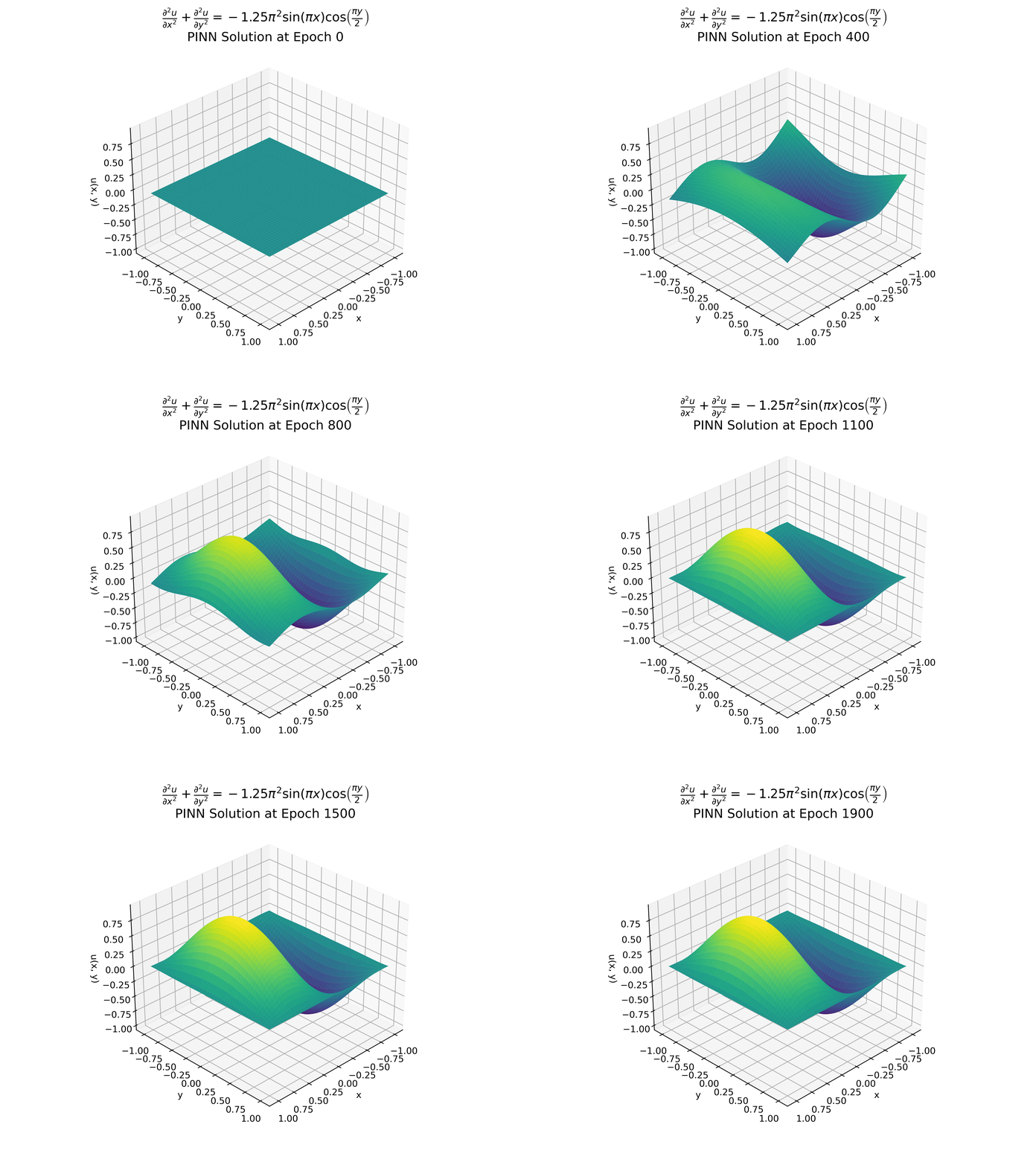
PINN solution for the Poisson equation over 2,000 epochs

Take a moment to watch the animation above. What you’re seeing isn’t just a model fitting to data points. It’s a neural network, starting from a random, chaotic surface, that is gradually being sculpted by a fundamental law of physics. It’s learning not just what a solution looks like, but why it must look that way.

This process is a glimpse into the fascinating field of Physics-Informed Neural Networks (PINNs), and it represents a conceptual leap from what we typically expect from AI.

For years, deep learning has been synonymous with pattern matching. We show a model thousands of cat photos, and it learns the statistical patterns of pixels that mean “cat.” It’s incredibly powerful, but it’s fundamentally about imitation. PINNs, however, go beyond pattern matching. Instead of just learning from a finished solution, we give the network an idea of the rules of the game — the governing physical equation — and ask it to construct the solution from scratch. In this post, I’ll guide you through a hands-on tutorial to build a PINN from scratch in PyTorch to solve the 2D Poisson equation.

The Problem — Our Law of Physics

Every PINN needs a physical law to enforce. For this project, we’ll use one of the most fundamental equations in physics and engineering: the Poisson equation, which models many kinds of steady-state phenomena, from the gravitational potential in space to the pressure field in a fluid. We can think of it in a more intuitive way: it describes the temperature distribution on a metal plate that has an internal heat source.

The equation is written as:

In this exercise we’ll solve the Poisson equation on a simple 2D square domain with the following conditions:

1. The Equation: We’ll use a specific source term f(x,y) that we've engineered:

Test PDE: Constructed using the Method of Manufactured Solutions

2. The Domain: A square where x ∈ [−1,1] and y ∈ [−1,1].

3. The Boundary Conditions: The value of u is fixed to zero on all four sides of the square. Think of this as the edges of our metal plate being held at a constant 0°C.

The true/analytical solution of our test PDE is:

Analytical Solution

The PINN Architecture

How do we get a neural network to solve our problem? The magic isn’t in a complex new model architecture; in fact, the model itself is surprisingly simple. The real innovation is in how we train it — specifically, how we design the loss function to teach the network the laws of physics.

The Model: A Simple Function Approximator:

The model we’ll use is a standard feed-forward neural network. You can think of it as a universal function approximator. Our goal is to find the weights and biases (θ) of this network such that its output, u​(x,y), becomes a good approximation of the true solution to our PDE.

• Input: A 2D coordinate, (x,y).
• Hidden Layers: Fully connected layers with smooth activation functions
• Output: A single scalar value, the predicted ‘u_pred’ at that coordinate.

The Loss Function: The Secret Sauce:

This is where the “physics-informed” part comes in. Instead of just training the network on a dataset of known (x,y) and u values, we train it on the physical constraints of the problem itself. We do this by creating a composite loss function with two distinct components:

1. The Boundary Loss: This is the easy part and feels like traditional supervised learning. We know for a fact that the solution u must be zero on the boundaries of our square. So, we enforce this by:
2. Sampling a set of points on the four boundary lines (x=±1, y=±1).
3. Calculating the Mean Squared Error (MSE) between the network’s predictions at these points and the true value, which is zero:

2. Physics Loss: This is the core of the PINN. We need to ensure that the solution inside the domain obeys our Poisson equation. We achieve this using the power of automatic differentiation, a feature built into PyTorch.
3. We sample a large number of random points, called “collocation points,” inside the domain.
4. For each point, we feed it through the network to get the output ‘u_pred’.
5. We then ask PyTorch to automatically calculate the second partial derivatives of the network’s output with respect to its inputs
6. We check how well these derivatives satisfy the governing equation. The difference is called the “residual”:

5. The physics loss is the Mean Squared Error of this residual. By forcing this loss to zero, we are forcing the network to satisfy the PDE.

The total loss is a weighted sum of these two components. By minimizing this single value, the network must learn to simultaneously satisfy the boundary conditions and the underlying physical law across the entire domain.

A Crucial Distinction: This is Not Supervised Learning:

It’s important to pause and realize what we are not doing. We are not providing the network with the true solution u(x,y) inside the domain and asking it to fit that data. That would be standard supervised learning—simple pattern matching.

Instead, the network is forced to discover the solution on its own. The only “supervision” it receives comes from the boundary conditions (the edges) and the physics loss (the rules). This is what makes the PINN approach so powerful: it can find solutions in scenarios where we don’t have labeled data, which is the case for most real-world physics and engineering problems.

The Implementation

Now, let’s translate the theory from Section 3 into practical PyTorch code. We’ll build the three core components: the network model, the loss calculation using automatic differentiation, and the training loop.

1. The Network Model

First, we define our neural network using torch.nn.Module. It's a simple feed-forward architecture that takes 2 input features (x, y) and produces 1 output feature (u). We will use siLU as our activation function, for calculating the derivatives needed for the physics loss.

[embed]

2. The Physics-Informed Loss Function

This is where the magic happens. We need to calculate the physics loss. The key is using torch.autograd.grad to compute the partial derivatives. I took inspiration from the clear and effective approach detailed in **Theo Wolf’s excellent post on Physics-informed Neural Networks**.

[embed]

The create_graph=True argument is the secret sauce. It tells PyTorch to build a computation graph for the first derivative, which allows us to back-propagate through it again to get the second derivative.

3. The Boundary Loss Function

[embed]

4. The Training Loop

Finally, the training loop is a standard PyTorch procedure. We calculate our combined loss, back-propagate, and update the model’s weights.

[embed]

Visualizing the Solution

First, let’s examine the final loss curve. It shows a steady and consistent decrease in both the physics and boundary losses throughout training — an encouraging sign of a healthy, convergent run. Notice that the physics loss remains significantly higher than the boundary loss across epochs. This imbalance suggests that the loss weighting coefficients (λ) need to be tuned while training to ensure a balanced contribution from both terms.

Loss curves

The Final Solution

The real proof, however, is in the final output. Since we chose a problem with a known analytical solution, we can directly compare our model’s prediction. Below is a three-panel comparison showing the result:

Let’s break down what we’re seeing:

1. PINN Solution (Left): This is the output of our trained neural network over the 2D domain. It’s a smooth, continuous surface that represents the function our model learned.
2. Exact Solution (Center): This is the ground truth, the plot of the analytical formula. Visually, it’s nearly identical to what our PINN discovered.
3. Error Map (Right): This is the most important plot. It shows the absolute difference between the exact solution and the PINN prediction, at every point. It can be seen that the error is quite small (on the order of 10−3).

The result is clear: our network didn’t just find an answer; it found the correct one. Without ever being shown the true solution, it leveraged the physical law encoded in the loss function to discover the underlying function on its own. This is the power of going “Beyond Pattern Matching.”

Conclusion — The Power and Promise of PINNs

The project we just walked through is more than just an academic exercise; it’s a demonstration of a powerful new paradigm in scientific computing. By successfully solving the Poisson equation, we’ve shown that neural networks can do more than just match patterns in data — they can learn to respect the fundamental laws of physics.

Why Does This Matter? The Power of “Soft Constraints”

The technique we used, adding the boundary conditions and the PDE residual to the loss function, is a form of a penalty method. Instead of being rigidly forced to obey the rules, the network is simply penalized during training for violating them. This “soft constraint” approach is the source of a PINN’s incredible flexibility. It allows us to incorporate different kinds of information in a single model. For example, we could easily add:

• Data from a few real-world sensor measurements.
• Multiple physical laws that must be obeyed simultaneously.
• Different types of boundary conditions on different parts of the domain.

This makes PINNs a powerful framework for tackling complex, multi-physics problems that are often challenging for traditional simulators.

What if We Don’t Know the Physics?

This also leads us to a question: what happens when we don’t know the underlying physics completely? This is where PINNs can truly shine and evolve from a PDE solver into a tool for scientific discovery.

We can think of models on a spectrum:

• Black-Box Models (Standard AI): Purely data-driven. They know nothing about the underlying physics.
• White-Box Models (Traditional Simulators): Purely physics-driven. They require the governing equations to be known perfectly.
• Gray-Box Models (PINNs): PINNs can operate anywhere in between.

Imagine a scenario where you have some sensor data from a system, but you only have a partial or incomplete PDE. With a PINN, you can create a loss function that combines three things:

1. A data loss to make the model fit your sensor measurements.
2. A physics loss for the parts of the PDE you do know.
3. Trainable parameters in the PDE representing the parts you don’t know.

In this way, the network can use the available data to learn the unknown parameters of your physical model. It’s a framework that seamlessly blends data and theory, allowing us to discover the governing laws of a system, not just solve them. This ability to fuse empirical data with physical principles is why the future of scientific computing is likely to be physics-informed.

Thank you for reading! I hope this has given you a clear and intuitive introduction to the PINNs. Feel free to leave comments or questions below, and you can find the complete, fully-commented code for this project on my GitHub Repository.