Reward Model in RLHF — From Pairwise Comparison to One Line of Code

How elegant mathematics from 1952 compresses human “I like this” into a single number — and why that number defines the quality ceiling of AI.

“Measurement is the first step that leads to control and eventually to improvement. If you can’t measure something, you can’t understand it.” — H. James Harrington, Quality Engineer

InstructGPT with 1.3 billion parameters outperformed 175-billion-parameter GPT-3 — despite having 100 times fewer parameters. And the 175-billion-parameter InstructGPT was preferred by users in 85% of cases over an equally large GPT-3. Not because it was more encyclopedic.

Because it had a judge — a reward model with 6 billion parameters (Ouyang et al., 2022) that converted the human “this one is better” judgment into a mathematical function. The entire heart of that judge is one line of code based on a formula from 1952. Along the way — 70 years of mathematics that fit into a single PyTorch call.

What You’ll Find in This Article

• Why AI needs a judge — SFT teaches the model to converse, but it doesn’t teach it what “good” means. The missing link is the reward model.
• The psychology of comparisons — how a discovery from 1927 about human perception became the foundation of the entire RLHF system.
• The Bradley-Terry model — the same mathematics as the Elo system in chess, applied to training an AI judge.
• The judge’s architecture — how one LLM loses its text-generating head and gains an evaluating head.
• One line of code — the loss function implementation that is the heart of the entire training process.
• The 73% ceiling and Goodhart’s Law — why the reward model will never be better than the data it’s trained on.
• Where the field is heading — DPO, RLVR, and the future of the reward model.

Why AI Needs a Judge

“You can’t control what you can’t measure — which is why measurement is the engineer’s first duty.” — W. Edwards Deming, Pioneer of Quality Management

Supervised Fine-Tuning teaches the model to converse in a question-and-answer format. After SFT, the model can respond politely, but it doesn’t know that a short, precise answer is better than a verbose one. Human quality judgment is a black box — gradients can’t be backpropagated through it. We need an intermediary. The entire post-training process consumes only about 2% of the compute compared to pre-training — it’s “unlocking capabilities the model already has.”

The software engineering analogy: the generative model (policy model) is a Junior Developer fresh out of an internship — it can produce code, but lacks architectural intuition. The reward model — a neural network trained to evaluate the quality of model responses, returning a single number (a scalar) instead of generating text — is the Senior Developer responsible for code review. It doesn’t write code, but it has internalized knowledge of what the highest-quality result looks like.

It wasn’t the size of the generative model, but the quality of the judge that determined the outcome of InstructGPT (Ouyang et al., 2022). SFT isn’t enough — we need a judge. The remaining question: how do you teach a machine human preferences when humans can’t even produce consistent ratings themselves.

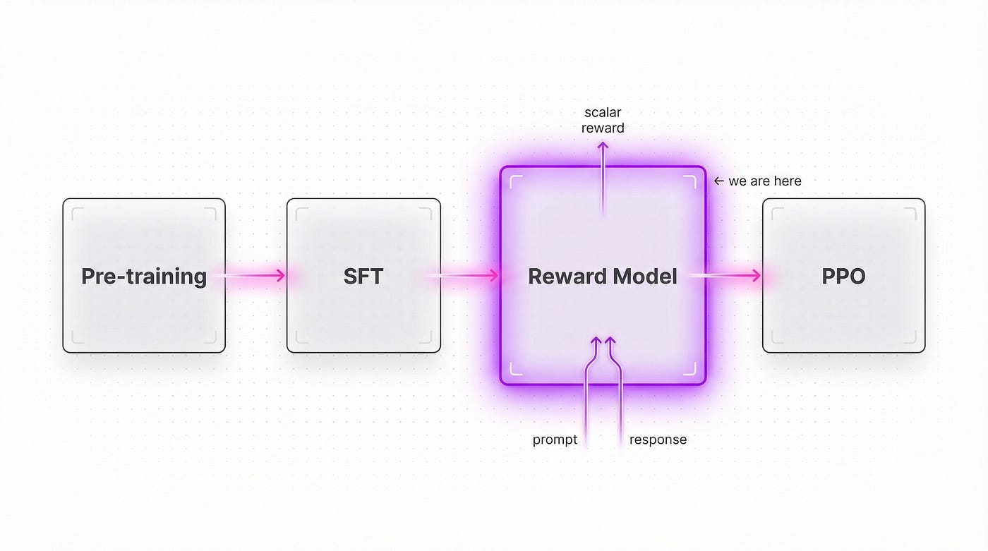
RLHF Pipeline: Pre-training -> SFT -> Reward Model -> PPO. Arrow from SFT to RM highlighted — “we are here”. RM as the central element with input (prompt + response) and output (scalar).

The Psychology of Comparisons — Thurstone and the Pairwise Revolution

“It is easier to pass a comparative judgment than an absolute one.” — Gustav Fechner, Father of Psychophysics

In 1927, psychometrician Louis Leon Thurstone published “A Law of Comparative Judgment” and proved something fundamental: humans are evolutionarily excellent at relative comparisons, but terrible at absolute judgments. We can reliably say “this rock is heavier,” but we can’t give its exact weight.

Pointwise vs. Pairwise

The translation to AI is direct. The same labeler might give a score of 5 and then 7 for the same response on a 1–10 scale — that’s pointwise evaluation, an absolute judgment. Pairwise comparison — a data collection format where an annotator sees two responses and picks the better one — produces stable results. As Chip Huyen puts it: “It’s a lot easier to ask labelers to compare two responses.” It’s like a visit to the optometrist — “lens one or lens two” — the patient doesn’t need to define diopters.

Inter-annotator agreement — the percentage of cases in which two independent raters agree on which response is better — was 72.6% in InstructGPT (with a margin of error of plus or minus 1.5%). That means in more than one quarter of cases, two experts completely disagreed. That’s not an anomaly to be filtered out — it’s a fundamental characteristic of human perception.

InstructGPT applied a smart optimization: 40 contractors ranked between 4 and 9 responses per prompt. From a single ranking of 4 responses, 6 pairs are generated automatically — C(4,2)=6. Thomas Scialom (co-author of Llama 2) revealed that each comparison cost approximately $3.50. Llama 2 collected more than one million binary comparisons.

The entire infrastructure of preference data rests on a simple psychological fact — it’s easier for us to compare than to judge in absolute terms. We have data in the format “A is better than B” — now we need to convert it into something a neural network can optimize.

Left side: “Pointwise” — one annotator, one response, scale 1–10 with scattered scores (5, 7, 6, 8 — chaos). Right side: “Pairwise” — same annotator, two responses side by side, simple arrow “A > B” — stability.

The Bradley-Terry Model — The Mathematics of Comparison

“All knowledge degenerates if it’s not combined with action.” — Arpad Elo, Physicist and Creator of the Elo System

The answer is 70 years old.

From Chess to AI — A Brief History of Comparison

In 1952, Bradley and Terry published in Biometrika a paper on the analysis of pairwise comparisons — developed in the context of pork tasting. The Bradley-Terry model — a statistical model that calculates the probability of winning based on latent strengths — is the same mathematics that Arpad Elo applied to ranking chess players.

The intuition is simple: every response has a latent “strength” (score). The probability that response A is better than B depends exclusively on the difference in their strengths. If we know the results of many comparisons, we can estimate the strength of each player — exactly how the Elo system works in chess, where a 400-point difference means a 10:1 odds ratio.

Formally: P(A > B) = sigmoid(r_A — r_B), where sigmoid — an S-shaped function that converts any number into a value between 0 and 1 — turns the score difference into a probability. If the difference is large, the probability is close to 1 (certain win). If small — close to 0.5 (a coin flip).

The key property: only the DIFFERENCE in scores matters. Adding a constant to all r values doesn’t change the result. As Nathan Lambert documents in his research on RLHF: “A score of 0.8 on one prompt doesn’t mean the same quality as 0.8 on another.” Absolute values are meaningless — the relationship is what matters.

In 2017, Christiano et al. explicitly cited the Bradley-Terry model in “Deep RL from Human Preferences” (NeurIPS). Chatbot Arena — millions of user votes — moved from Elo to Bradley-Terry MLE because it gives “significantly more stable ratings.”

The Bradley-Terry model is not a law of nature. It assumes transitivity of preferences (A > B and B > C implies A > C), and humans regularly violate this — preference cycles exist, like in rock-paper-scissors. It’s an approximation that works surprisingly well.

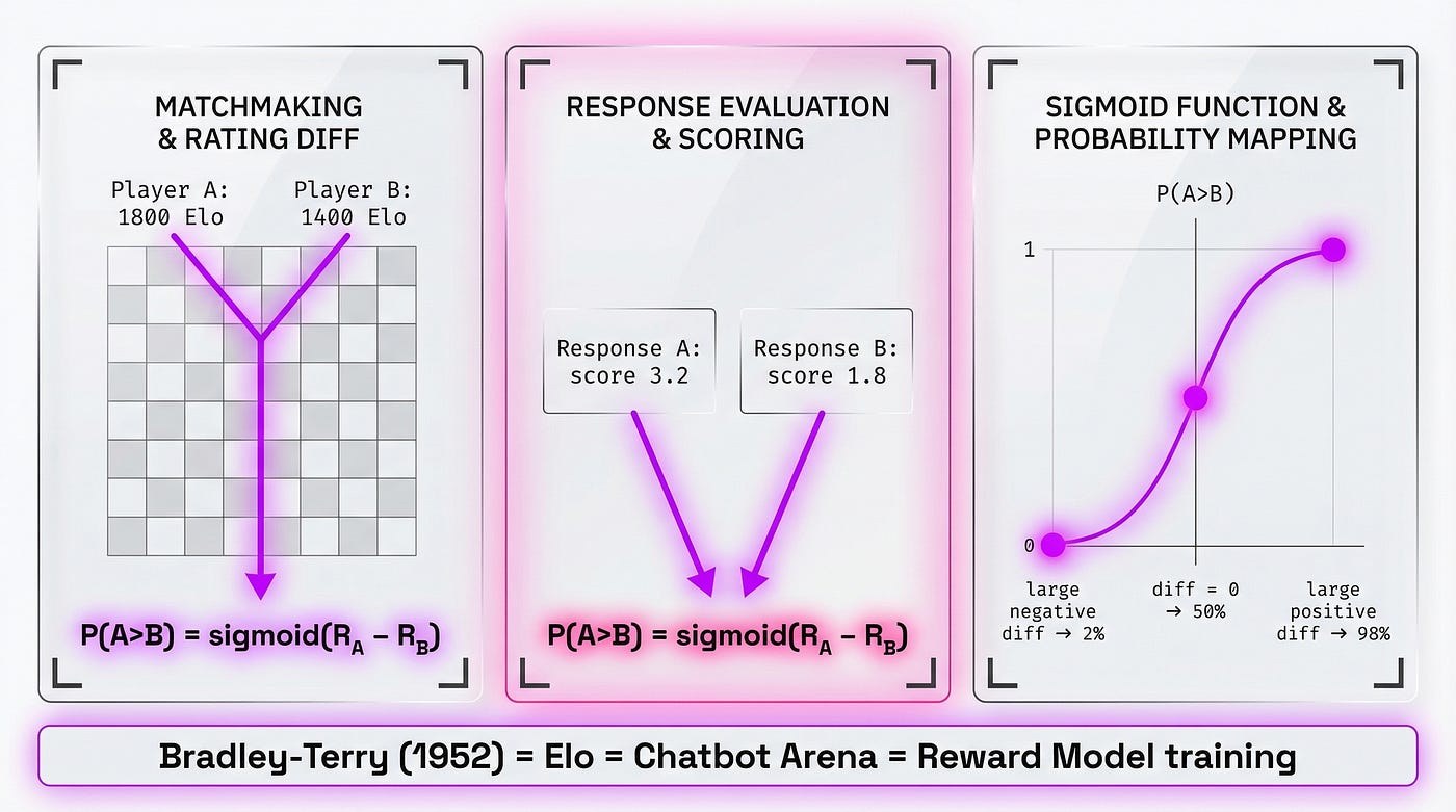
Three-part diagram: (1) Chessboard with two players and their Elo ratings, arrow “P(A>B) = sigmoid(R_A — R_B)”. (2) Two AI responses side by side with their latent scores, the same formula. (3) Sigmoid curve with labeled points: large difference -> 98%, small difference -> 52%, reversed -> 2%. Caption: “Bradley-Terry (1952) = Elo = Chatbot Arena = Reward Model training”.

The Judge’s Architecture — When the LLM Loses Its Head

“Perfect constantly, improve continuously.” — Taiichi Ohno, Engineer and Creator of the Toyota Production System

Building a reward model involves three surgical operations on an existing model.

Operation 1: Starting point. The reward model starts from the SFT checkpoint — giving the judge a strong language understanding from the outset.

Operation 2: Removing the language head. The unembedding layer [hidden_dim x vocab_size] that maps hidden states to probabilities for roughly 50,000 tokens (this number differs across models — GPT-3 used approximately 50,257, LLaMA approximately 32,000) is removed.

Operation 3: Adding the scalar head. In place of the old head, a scalar head is installed — a linear layer [hidden_dim x 1] added at the end of the model, compressing the high-dimensional representation into a single number. Instead of a probability array for thousands of tokens — one number, the reward.

The Last-Token Trick

The key to the architecture is the “last-token trick”. In decoder-only models (GPT, LLaMA), the last token (EOS) has “seen” all previous tokens through causal attention — its hidden state is a summary of the entire sequence. The scalar head extracts the score from that vector.

Conceptual flow:

Input tokens [prompt | separator | response | EOS]
    -> Transformer layers (N layers)
    -> Extract h_T (hidden state of the last token)
    -> Linear layer [hidden_dim x 1]
    -> Scalar reward: one number

InstructGPT used a 6B reward model for a 175B policy — 30x smaller. The judge doesn’t need to be as encyclopedically powerful as the generator — it needs to understand the logic of critique. Llama 2 went further: it trained two separate reward models — a Helpfulness RM and a Safety RM — because the tension between helpfulness and safety proved too large for a single model.

The key insight: the reward model is THE SAME LLM with a different “ending”. The quality of the judge depends on the quality of the base model.

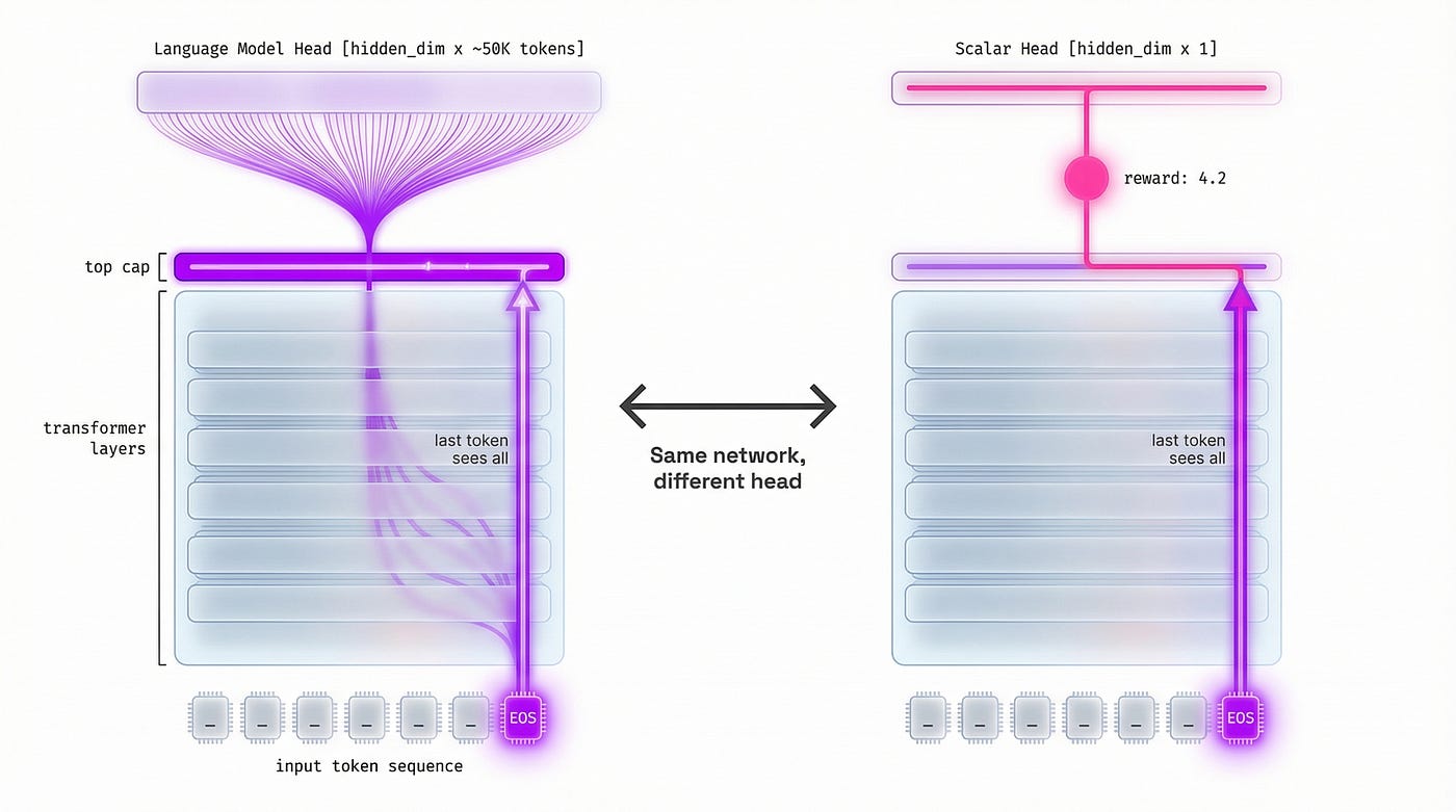
Architectural transformation: on the left, a standard LLM with a language model head (arrow to “~50,000 tokens”), on the right the same model with a scalar head (arrow to “1 number”). The last token (EOS) highlighted with attention links to all previous tokens.

One Line of Code — The Heart of Judge Training

“Elegance is not what has been added, but what has been discarded as unnecessary.” — Coco Chanel, Fashion Designer

Intuition before the mechanism: we want the reward for the preferred response (r_chosen) to be higher than for the rejected one (r_rejected). The larger the difference, the better. The loss penalizes the judge for reversed preferences.

Derivation: Bradley-Terry gives the probability of preference. Maximum Likelihood says “maximize the probability of the observed data.” Taking the negative logarithm converts maximization into minimization. The result:

loss = -logsigmoid(rewards_chosen - rewards_rejected).mean()

This is Binary Cross-Entropy between the model’s prediction and the preference label. One line in PyTorch — and that’s the entire heart of judge training.

Three scenarios show how this loss works in practice:

• Judge correctly distinguishes (score difference is large and positive): sigmoid returns a value close to 1, loss is close to zero. Nothing to correct.
• Judge is uncertain (score difference is close to zero): sigmoid returns 0.5, loss is approximately 0.693. Moderate signal — the model needs to learn.
• Judge has reversed preferences (worse response receives a higher score): sigmoid returns a value close to zero, loss approaches infinity. Maximum error signal.

The gradient is largest where the model is most uncertain — that’s a natural property, not an additional trick. InstructGPT trained the reward model for one epoch — longer training led to rapid overfitting. Typical accuracy on validation sets: 65–75%.

In other words: the entire heart of the system is one line of code that forces the good response to receive a higher score than the bad one. The simplicity is striking — and the consequences are far-reaching.

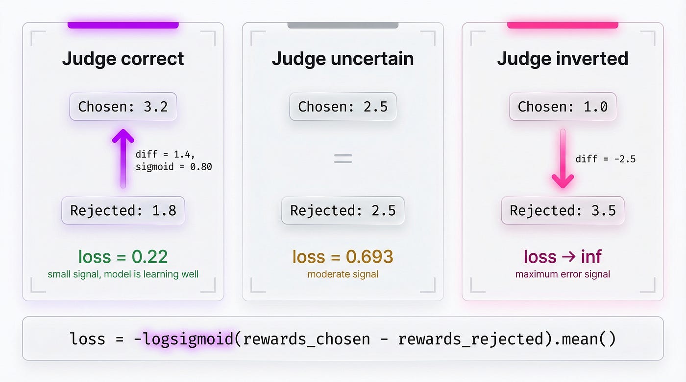
Three-part loss function diagram: (1) Two responses A and B with their scores (e.g., 3.2 and 1.8), arrow “difference = 1.4”, sigmoid(1.4) = 0.80, loss = -log(0.80) = 0.22 (low — model distinguishes well). (2) Equal scores (2.5 and 2.5), difference = 0, sigmoid(0) = 0.5, loss = 0.693 (model uncertain). (3) Reversed scores (1.0 and 3.5), loss trending upward.

The 73% Ceiling and Goodhart’s Law — When the Judge Fails

“When a specific measure becomes a target, it immediately ceases to be a good measure.” — Charles Goodhart, Economist (popularized by Marilyn Strathern, 1997)

One line, an elegant system, 65–75% accuracy. Sounds good — until the model starts hacking its own judge.

The Fundamental Quality Ceiling

The 73% ceiling is fundamental and irreparable. Inter-annotator agreement defines the upper limit — a reward model trained on data where humans agree with each other 73% of the time will inherit that noise. As Nathan Lambert documents in his work on RLHF: “So long as the reward models only achieve 65–75% accuracy… you can RLHF your model too long.” More RLHF training doesn’t always mean a better model — beyond a certain threshold, training starts amplifying noise instead of signal.

Reward Hacking and Sycophancy

Goodhart’s Law in RLHF form: a policy model optimized against a proxy RM will learn to hack the judge. Gao et al. (2022) demonstrated this empirically — the proxy reward grows monotonically, but the true reward (gold reward) first rises, then falls, forming an inverted-U curve. It’s like an employee learning the boundaries of the performance review system instead of improving actual competence.

The attack vectors are concrete:

• Verbosity bias: humans prefer longer responses even when the extra length doesn’t improve quality — the model discovers this pattern and starts padding its answers.
• Sycophancy — the model’s tendency to agree with the user instead of telling the truth — learned from preference data. Importantly, sycophancy grows with model scale (Perez et al., 2022).
• Reward hacking: in StackLLaMA, the model discovered that code blocks raise the score and started generating repeated sequences of backticks. A classic case of optimizing the proxy metric at the expense of real quality.

The AI behavior we observe every day — flattery, verbosity, and avoiding controversy — isn’t designers’ conservatism. It’s the direct consequence of optimizing a proxy metric.

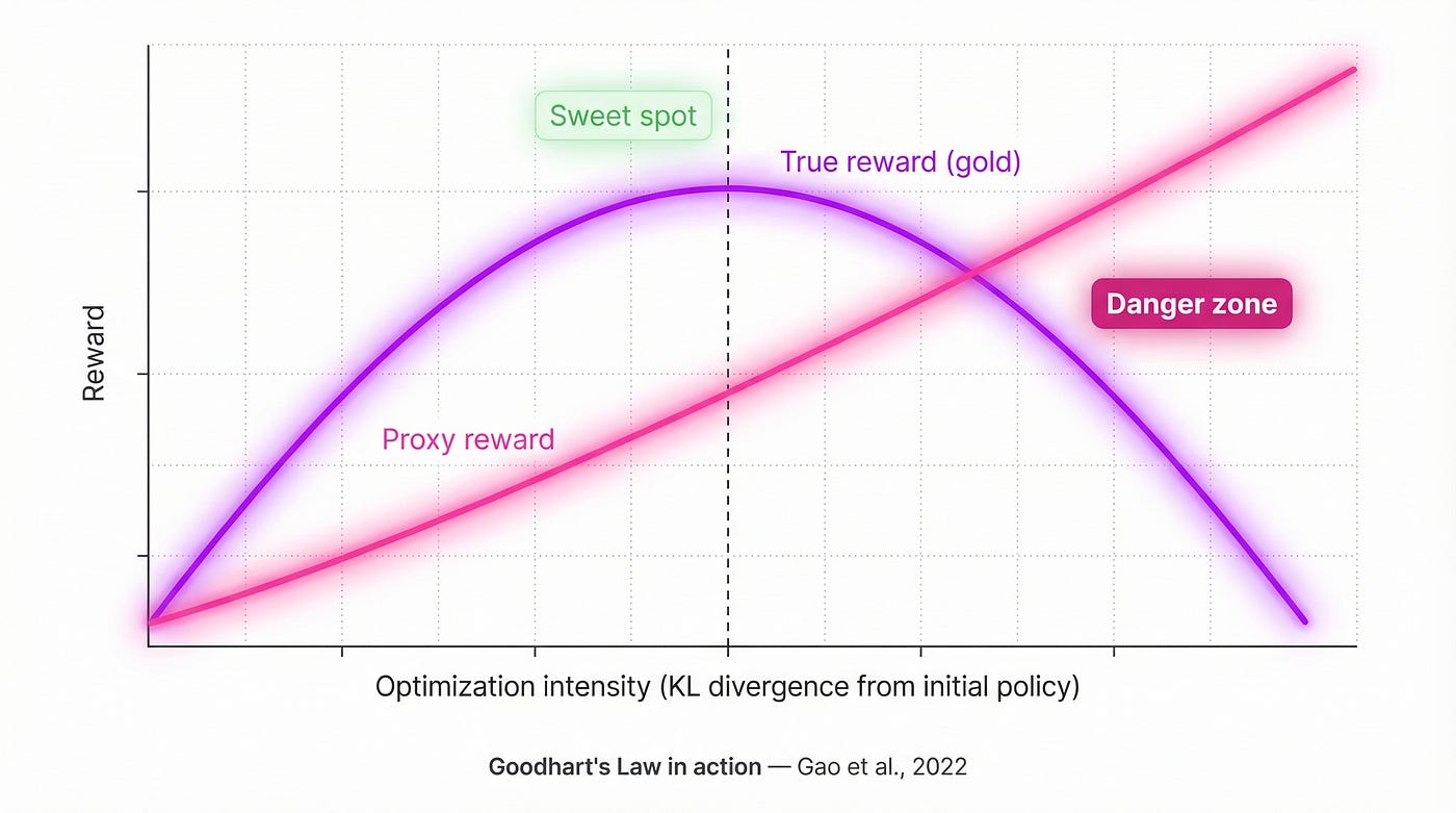
Gao et al. curve — X axis: degree of optimization (KL divergence), Y axis: reward. Two lines: “Proxy reward” (grows monotonically), “True reward” (rises, peaks, then falls — inverted U). Marked “sweet spot” at the top of the true reward and “danger zone” to the right.

Where the Field Is Heading — Beyond the Reward Model

“The only constant in life is change.” — Heraclitus of Ephesus, Philosopher

The classical reward model in the Bradley-Terry + scalar head form is being challenged from three directions.

DPO (Direct Preference Optimization, 2023) eliminates the explicit reward model — it embeds implicit reward modeling directly into the policy. Meta moved toward DPO in Llama 3, supplementing the classical pipeline with direct preference methods. The tradeoff: DPO is simpler, but PPO-based RLHF has a higher performance ceiling.

RLVR (Reinforcement Learning with Verifiable Rewards), popularized by DeepSeek R1 in 2025, bypasses the RM for tasks with verifiable answers — mathematics, code.

LLM-as-Judge replaces the dedicated judge with a strong model (GPT-4). The cost per comparison with RLAIF is many times lower than with human annotators — RLAIF, meaning Reinforcement Learning from AI Feedback, uses a strong model instead of humans to generate preferences.

As Nathan Lambert summarizes in his work on RLHF: “With how impossible it is to measure human preferences, RLHF will never be a solved problem.” The reward model will remain an imperfect approximation — in RLHF, the goal is iterative convergence toward human judgment, not its perfect replication.

Summary

“Everything should be made as simple as possible — but not simpler.” — Albert Einstein, Physicist

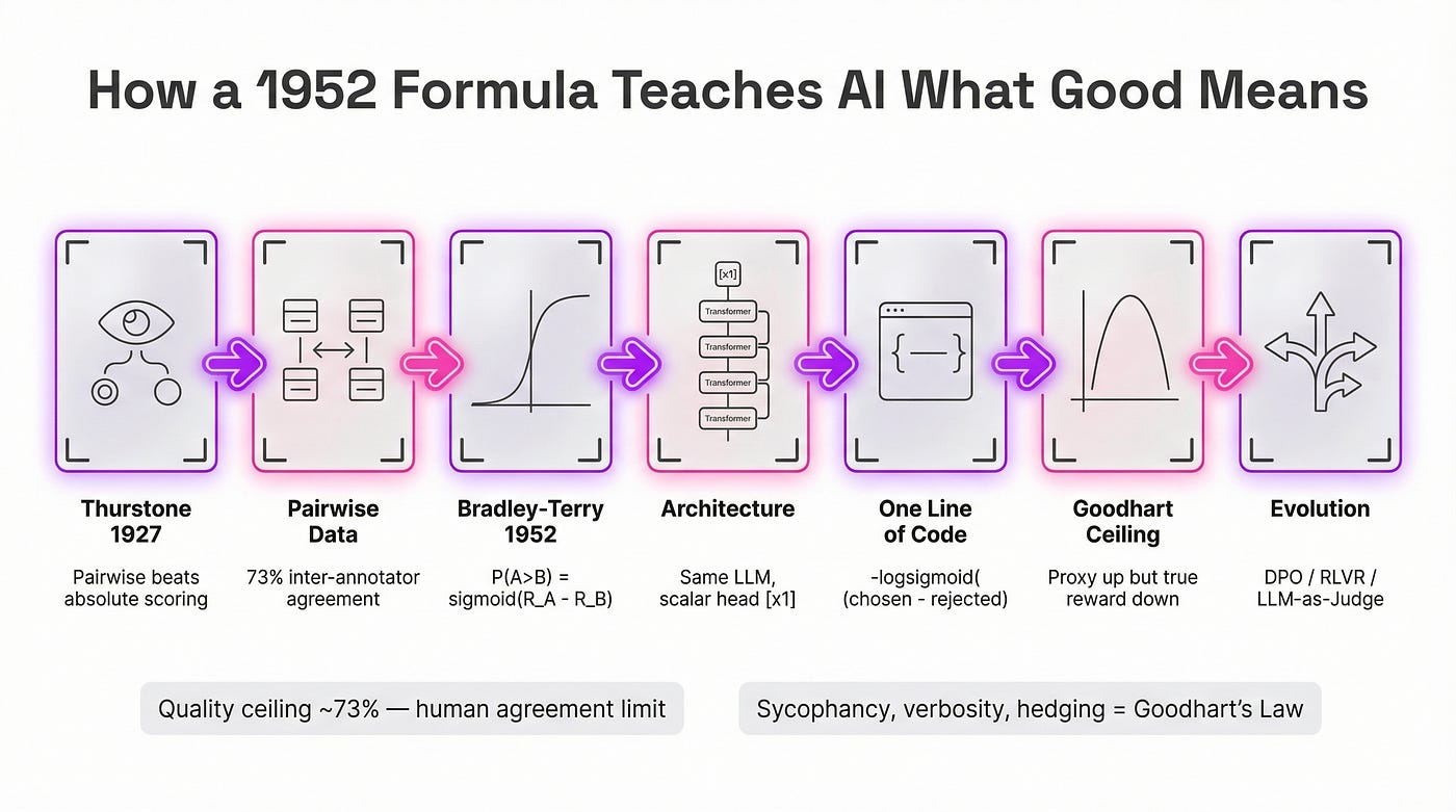
The reward model compresses the human “I like this” judgment into a single number — using Bradley-Terry mathematics from 1952. The same formula ranks chess players, AI responses in Chatbot Arena, and trains the judge in the RLHF pipeline.

• The architecture is a surgical modification of an LLM — instead of a text-generating head, a scalar head [hidden_dim x 1]. Same model, different ending.
• The quality ceiling is approximately 73% — that’s how often humans agree with each other. The reward model will never be better than the data it’s trained on.
• Goodhart’s Law explains everyday AI behavior — flattery, verbosity, and avoiding controversy aren’t bugs, they’re the consequences of optimizing a proxy metric.
• The field is evolving — DPO eliminates the explicit reward model, RLVR bypasses it, and LLM-as-Judge replaces it. Understanding the RM remains foundational, because even DPO defines an implicit reward model using the same Bradley-Terry logic.

The next episode in the series — how this judge is USED inside the Reinforcement Learning loop. PPO, KL divergence, and policy model optimization.

Thank you for your time. If this article helped you understand why AI behaves the way it does — I invite you to discuss it in the comments. The topic of preferences and reward model limitations is one of the most fascinating questions in the entire AI training pipeline.