Time and Space Complexity: The Backbone of Efficient Algorithms

Time and Space Complexity

Introduction

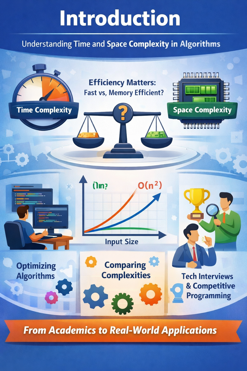
In the modern era of technology, efficiency plays a vital role in the success of any software system. From mobile applications to large-scale enterprise systems, users expect fast responses and seamless performance. Behind this efficiency lies a fundamental concept in computer science known as time and space complexity. These concepts help in evaluating how well an algorithm performs when the size of the input increases.

When solving a problem, there can be multiple ways to write an algorithm. However, not all solutions are equally efficient. Some may take more time, while others may consume excessive memory. This is where time and space complexity become essential — they allow developers to compare different approaches and select the most optimal one.

Understanding these concepts is not only important for academic purposes but also crucial in real-world applications, competitive programming, and technical interviews.

Understanding Time Complexity

Time complexity measures how the execution time of an algorithm increases with the size of the input. Instead of focusing on exact time (which depends on hardware and system conditions), it focuses on the growth rate of the algorithm.

Time complexity is usually expressed using Big-O notation, which represents the worst-case scenario. This helps developers prepare for the most demanding situations.

Common Types of Time Complexity

• O(1) — Constant Time The algorithm executes in the same time regardless of input size. Example: Accessing an element in an array using its index.
• O(n) — Linear Time The execution time increases linearly with input size. Example: Searching for an element using linear search.
• O(log n) — Logarithmic Time The execution time increases slowly as the input size grows. Example: Binary search, where the dataset is repeatedly divided into halves.
• O(n log n) — Linearithmic Time Common in efficient sorting algorithms. Example: Merge sort and quick sort (average case).
• O(n²) — Quadratic Time Execution time increases rapidly due to nested loops. Example: Bubble sort, selection sort.
• O(2ⁿ) — Exponential Time Extremely slow and inefficient for large inputs. Example: Recursive solutions for Fibonacci without optimization.

Understanding Space Complexity

Space complexity refers to the amount of memory required by an algorithm as a function of input size. It includes both:

• Input Space: Memory used to store the input
• Auxiliary Space: Extra memory used by the algorithm

Efficient programs aim to use minimal memory while maintaining good performance.

Examples of Space Complexity

• O(1): Using a fixed number of variables
• O(n): Creating additional arrays or data structures
• O(n²): Using matrices or 2D arrays

For example, an algorithm that stores all elements in a new array will consume more memory compared to one that modifies data in place.

Big-O Notation: A Standard for Comparison

Big-O Notation: A Standard for Comparison

Big-O notation provides a standardized way to express algorithm efficiency. It focuses on how an algorithm behaves as the input size becomes very large.

Why Big-O Matters

• Helps compare different algorithms
• Predicts performance for large inputs
• Guides optimization decisions

Illustrative Example

Consider finding a number in a sorted list:

• Linear Search: Checks each element one by one → O(n)
• Binary Search: Divides the list repeatedly → O(log n)

As the dataset grows, binary search becomes significantly faster than linear search.

Best Case, Worst Case, and Average Case

Best Case, Worst Case, and Average Case

When analyzing an algorithm, its performance can change depending on the input. To understand this, we consider three cases:

• Best Case: This is the fastest scenario, where the algorithm takes the least time. Example: In linear search, when the element is found at the first position → O(1).
• Worst Case: This is the slowest scenario, where the algorithm takes the maximum time. Example: In linear search, when the element is at the last position or not present → O(n).
• Average Case: This represents the expected performance for random input. Example: In linear search, the element is usually found in the middle → O(n).

👉 Important: Developers mainly focus on the worst case because it ensures the algorithm performs reliably even in the most difficult situations.

Real-World Applications of Complexity Analysis

Real-World Applications of Complexity Analysis

Time and space complexity are widely used in real-world systems:

1. Search Engines

Search engines process billions of queries efficiently using optimized algorithms with low time complexity.

2. Navigation Systems

Applications like maps use algorithms to find the shortest path in minimum time.

3. E-commerce Platforms

Websites handle large volumes of users and transactions, requiring efficient algorithms to maintain performance.

4. Social Media Applications

Platforms manage huge datasets, including posts, likes, and messages, using optimized storage and retrieval techniques.

5. Banking Systems

Secure and fast processing of transactions relies heavily on efficient algorithms.

Common Mistakes to Avoid

While learning time and space complexity, students often make these mistakes:

• Ignoring worst-case scenarios
• Confusing time complexity with actual execution time
• Overlooking space complexity
• Using inefficient algorithms for large inputs

Avoiding these mistakes can significantly improve problem-solving skills.

Tips to Improve Algorithm Efficiency

• Choose the right data structure
• Avoid unnecessary nested loops
• Use recursion wisely (and optimize with memoization if needed)
• Analyze complexity before implementing
• Practice solving problems with optimized approaches

Diagram Placement Suggestions

To enhance your article visually, include diagrams at these points:

1. After Time Complexity Section 👉 Graph comparing O(1), O(log n), O(n), O(n²)
2. After Big-O Notation Section 👉 Linear search vs binary search comparison diagram
3. After Time-Space Trade-off Section 👉 Visual representation of speed vs memory usage

Conclusion

Time and space complexity are the backbone of efficient algorithm design. They provide a systematic way to evaluate and compare different solutions, ensuring that programs perform well even with large inputs.

In a world where speed and efficiency are critical, understanding these concepts is a must for every programmer. Whether developing applications, preparing for interviews, or solving real-world problems, mastering time and space complexity helps in writing optimized and scalable code.

By continuously practicing and analyzing algorithms, developers can improve their problem-solving skills and build high-performance systems that meet modern technological demands.