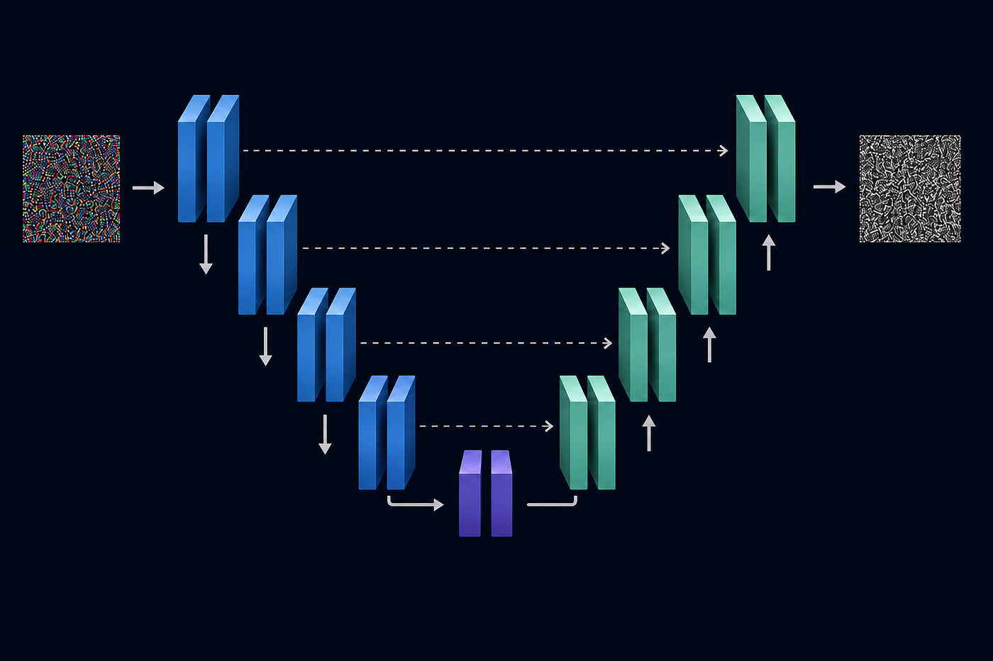
High level representation of a U-Net

Diffusion U-Net — Architecture and Building Blocks

1. Introduction

In a previous article we talked about Denoising Diffusion Probabilistic Models (DDPM) and the math behind it. We also quickly introduced the classic architecture used in the paper but without really going into detail yet. The goal of this article will be to code together a Diffusion U-Net, using its main building blocks.

To keep the article focused on the U-Net, for now we’ll treat components such as ResNet Blocks, Attention and Positional Embeddings as black boxes. Since each of those deserves an article of its own.

Pixel Space vs Latent Space

One more premise that I feel I should make is that our domain is currently the one of pixels, called Pixel Space. This means that our network will be input with images that are not being encoded. This works very well for small images (32x32 or 64x64) but starts to get computationally too expensive when training with images having a bigger size.

If you wished to train your model and generate images at higher resolutions you should first encode them in what’s called Latent Space, just like models like Stable Diffusion or Dall-E do.

2. Why a U-Net

This is a very natural question to ask, there are many architectures outside, and some of them are even more effective than U-Nets (side-eye to Transformers) in certain situations. But why initially was U-Net the architecture of choice?

This architecture was originally introduced for medical image segmentation, where the goal was accurate pixel prediction. At the same time Diffusion models require predicting noise distributed over an entire image — those same properties made the U-Net the natural choice.

U-Nets are also very flexible. Since they are mainly built using Conv2d layers they can process images at various resolutions, whether the input is 32x32 or 512x512. By progressively downsampling the feature maps, the spatial resolution is halved at each layer, while the number of channels increases. This dramatically reduces the number of feature values the network needs to process - from 512x512x3 to, for example, 8x8x512 - making the computation much more efficient, while increase the network's representational capacity.

After shrinking the image to extract all the information needed, the architecture needs to reconstruct it back to its original size. To do it, it was necessary to use another important tool: skip connections. Another reason why the U-Net is such a good fit for diffusion models.

Architecturally speaking the network consists of the following main sections:

• A Starting convolutional block
• A Down block
• A Bottleneck block
• An Up block
• An Ending convolutional block

3. Skip Connections

I think this is a topic that deserves a little section here in this specific article because without them the U-Net wouldn’t be what it actually is.

If you think of a U-Net, it is not very different from the idea behind an Encoder-Decoder architecture: the image shrinks while increasing in depth, and then it goes back to its original size and channel dimension.

What defines the U-Net is the use of Skip Connections connecting the encoding layers to the respective decoding ones.

Every time the image is downsampled, some spatial information is inevitably lost. By the time it reaches the bottleneck, the model has learned a rich semantic representation of the image, but lost many precise details, such as edges, textures or object boundaries. Skip connections solve this problem by directly passing that information from one layer of the encoder, to the corresponding layer of the decoder. The image will be decoded using global details, learned in the bottleneck, and those precise small details received back from the skip connections.

4. Starting Convolutional Block

This is an initial block used to project the image channel size to the U-Net starting channels. A 3-channels image is not a very rich feature representation, that’s why we want to enrich it by increasing the number of initial channels.

Very simply we define the conv2d main attributes:

• in_channels = 3 - our tensor's number of channels, usually 3: R, G, B.
• out_channels - this is the starting number of channels in our U-Net, 64 are a good start, but they can be increased.
• kernel_size = 1 - pointwise convolution to project channels without mixing information from the neighboring pixels. You could use a kernel_size = 3 to already start extracting local spatial features, but right now we only want to project channels.
• padding = 0 - since the filter is just 1x1 we don't need padding.

import torch

start_conv = nn.Conv2d(in_channels = 3, 
                       out_channels = 64,
                       kernel_size = 1,
                       padding = 0)

5. Down Block

This is the encoder of our U-Net, early stages learn local structures such as edges and textures, later stages learn higher-level semantic information and long range relationships. All while the image’s height and width get reduced and the channel size increases.

Each layer of the U-Net is made up of the following components:

• ResNet blocks
• Attention block
• Group normalization
• Skip connections
• Downsample / Upsample block

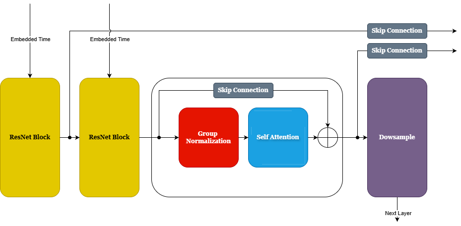
Architecture of the Down block

In each layer of the down path our model first processes the feature map while keeping the number of channels fixed. The ResNet blocks improve the image representation at the current resolution while the Attention block allows each spatial location to interact with other ones. This helps to model what is known as long-range dependencies. At the end of this block chain we downsample the image, compressing the feature map and increasing the receptive field by the defined channel multiplier.

While Attention is not required in each layer and you can experiment by adding it or removing it, ResNet blocks are a must and must not be forgotten...otherwise our network will look, well... kind of empty.

One thing to keep in mind is that time embeddings must be injected in each ResNet block, otherwise our model will never know what timestep that noise was coming from.

To avoid hardcoding channels we can decide a list of channel_multipliers that will increase our tensor number of channels: e.g. starting from 64 -> 128 -> 256 -> 512.

Notice that channels in each layer will stay constant: this is because each layer will specialize in learning features at specific spatial resolutions.

import torch
from torch import nn

base_dim = 64 # Base channels after start_conv
channel_multiplier = (1,2,4,8)
use_attention = (False, False, True, True)

# Creating a list of channels -> [64, 64, 128, 256, 512]
channel_list = [base_dim, *map(lambda m: m*base_dim, channel_multiplier)]
# In - Out channels list of tuples -> [(64, 64), (64, 128), (128, 256), (256, 512)]
in_out = list(zip(channel_list[:-1], channel_list[1:]))

# Create down list
down = nn.ModuleList([])
for i, (in_c, out_c) in enumerate(in_out):
 down_block = nn.ModuleList([
      ResNet(in_channels = in_c, 
             out_channels = in_c, 
             t_emb_dim = t_emb_dim),
      ResNet(in_channels = in_c, 
             out_channels = in_c,
             t_emb_dim = t_emb_dim)])

 # Use attention if required
 if use_attention[i]:
  attn = Residual(Groupnorm(SelfAttention(in_c)))
 else:
  attn = nn.Identity()

 # Divide feature size by half if it's not the last layer
 if i < (len(in_out)-1):
  downsample = Downsample(in_channels = in_c,
                          out_channels = out_c)
 else:
  downsample = nn.Conv2d(in_channels = in_c,
                         out_channels = out_c,
                         kernel_size = 3,
                         padding = 1)

 down_block.append(attn)
 down_block.append(downsample)

 down.append(down_block)

Notice that the last layer will not have a Downsample block, but just a nn.Conv2d layer. This is because we don't want to reduce the feature dimensions more before reaching the bottleneck, otherwise our tensor will be too tiny (e.g. 2x2) and very little information would remain.

Groupnorm and Residual

Those two are pretty small wrapper modules to add modularity to our network:

• Groupnorm — adds Group Normalization before a block - a more stable normalization technique than batch normalization when having smaller mini batches.
• Residual — adds a skip connection over a function to help gradients flow through deeper networks and avoid the vanishing gradients problem.

import torch
from torch import nn

class Groupnorm(nn.Module):
 "Applies GroupNorm before the specified function -> fn(norm(x))"
 def __init__(self, fn):
  super().__init__()
  self.fn = fn
  # num_groups and num_channels are hyperparameters you can tune
  self.norm = nn.GroupNorm(num_groups = 8, num_channels = 64)

 def forward(self, x, *args, **kwargs):
  return self.fn(self.norm(x), *args, **kwargs)

class Residual(nn.Module):
 "Adds a skip connection to the function -> x + f(x)"
 def __init__(self, fn):
  super().__init__()
  self.fn = fn
 def forward(self, x, *args, **kwargs):
  return x + self.fn(x, *args, **kwargs

Downsample

This is the block used to downsample our image from one resolution to the other all while dividing in half its spatial resolution. We have a couple of ways of doing so. Differently from the original DDPM, I like using a technique called Space-to-Depth Downsampling which helps preserving information by rearranging neighboring values to the channel dimension. That preserved information is then fed into a convolutional layer that learns how to combine it.

Another approach would be to use strided convolutions or pooling layers — those methods preserve less information by discarding some of it when they are applied.

import torch
from torch import nn

class Downsample(nn.Module):
 def __init__(self, in_channels, out_channels):
  super().__init__()
  self.conv = nn.Conv2d(in_channels = in_channels * 4,
                        out_channels = out_channels,
                        kernel_size = 1)

 def forward(self, x):
  B, C, H, W = x.shape # (128, 64, 32, 32)
  x = x.reshape(B, C, H//2, 2, W//2, 2) # (128, 64, 16, 2, 16, 2)
  x = x.permute(0,1,3,5,2,4) # (128, 64, 2, 2, 16, 16) 
  x = x.reshape(B, C * 4, H//2, W//2) # (128, 256, 16, 16)
  return self.conv(x) # (128, out_channels, 16, 16)

Time Embeddings

I know this topic will require an article of its own, but I still need to talk about it here. Otherwise our U-Net will never be complete without it!

Imagine I gave you two noisy images and asked: “Which one is noisier?” You would probably answer correctly without much difficulty.

Now imagine I showed you a noisy image and asked: “Can you remove exactly the amount of noise corresponding to timestep 700?” That would be much harder, because you don’t know how much noise timestep 700 represents.

That’s exactly the problem our U-Net has. Without knowing the current timestep, it has no idea how much noise is expected in the input image or how much it should remove. This is why we provide the timestep as an additional input to every ResNet block.

Of course, a single number like 700 doesn't carry much information for a neural network. To make it more expressive, we first encode it using a sinusoidal embedding—originally introduced in the Transformer paper—and then pass it through a small MLP before injecting it into the network in each ResNet block, conditioning the entire network on the current timestep.

import torch
from torch import nn

time_mlp = nn.Sequential(SinPositionalEmbedding(timesteps),
                         nn.Linear(in_features = base_dim,
                                   out_features = base_dim * 4),
                         nn.GELU(), # or SiLU()
                         nn.Linear(in_features = base_dim * 4, 
                                   out_features = base_dim))

Why do we use GELU() or SiLU() as activation functions? Why not the classic ReLU()? If you remember ReLU() is hard gated: x = max(0, x) which means that even small negative values get zeroed out completely. Functions like GELU() or SiLU() are soft gates. They are continuous when x = 0 and provide smoother gradients during optimization. They are usually preferred in Transformers or Diffusion models.

6. Bottleneck

Here we reached the deepest layer of our network. This is where features encode large portions of the image.

The nice part about this bottom layer is that the spatial resolution is pretty small…like, way smaller than what it started…hence…it’s definitely Self Attention time!!!

Here the number of channels is at its peak and since the spatial resolution is small we are not afraid of that O(n^2) computational cost of Self Attention, yay!

This block too has a pretty straightforward structure:

• ResNet block
• SelfAttention
• ResNet block

Modern diffusion U-Nets repeat this sequence multiple times. For the sake of simplicity we will only use one.

import torch
from torch import nn

bottle_dim = channel_list[-1] # e.g. 512

bottle = nn.ModuleList([
     ResNet(bottle_dim, bottle_dim, time_emb_dim),
     Residual(Groupnorm(SelfAttention(bottle_dim))),
     ResNet(bottle_dim, bottle_dim, time_emb_dim)
     ])

7. Up Block

This is where the image will start getting reconstructed until the final top layer. This is an exact mirror of the Down block but with a critical addition: now each stage will also receive the previous skip connections from the Down block. To construct it we will reverse the in_out list, thus creating a list of tuples that start from the highest number of channels (e.g. 512), to the lowest (e.g. 64).

Remember that now we need to concatenate the skip connections too before each ResNet block, therefore its in_channel will have size equal to the sum of the input and output dimension! To be more clear, let's take a channel (in_c, out_c) tuple, for example (128, 256). In the Down path we stored the tensor when it had a channel size equal to 128 (remember that it’s expanded to 256 channels following the Downsample block); in the Up path these channel pairs will be reversed, hence we will have (256, 128). Since we want to add the skip connection we will need to set the in_channels equal to 256+128! Done!

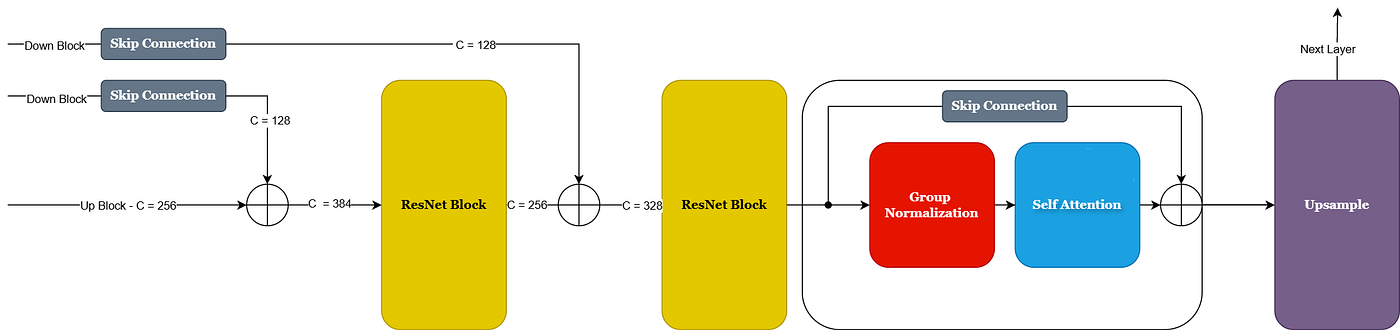
Architecture of the Up block

import torch
from torch import nn

up = nn.ModuleList([])

# What layers attention should be added at
use_attention = (False, False, True, True)

for i, (out_c, in_c) in enumerate(reversed(in_out)): # outputs [(256, 512), (128, 256), ...]
 up_block = nn.ModuleList([
                  ResNet(in_ch+out_c, in_c, time_emb_dim),
                  ResNet(in_c+out_c, in_c, time_emb_dim)
                  ])

 # Use attention if required
 if use_attention[len(use_attention) - 1 - i]: 
  attn = Residual(Groupnorm(SelfAttention(in_c)))
 else:
  attn = nn.Identity()

 # Double the spatial resolution if it's not the topmost layer
 if i < (len(in_out) - 1):
  upsample = Upsample(in_channels = in_c, 
                      out_channels = out_c)
 else:
  upsample = nn.Conv2d(in_c, out_c, kernel_size = 3, padding = 1)

 up_block.append(attn)
 up_block.append(upsample)

 up.append(up_block)

Upsample

This is the block that will help turn our image back to its original size. We will use the functional.interpolate to avoid ConvTranspose2d. Interpolate mathematically generates pixels and if followed by a convolutional layer with a 3x3 kernel will add the learnability of a convolutional layer while adapting the number of channels.

ConvTranspose2d is learnable, but it has the drawback to possibly add checkerboard artifacts to the image.

As for the interpolation mode we can use nearest, it’s computationally faster than other interpolation methods. Its downside is that it adds some uneven edges to the image. Other interpolation methods we could use are bilinear or bicubic . They produce better outputs when decoding, but they are computationally more expensive and slower.

import torch
import torch.nn.functional as F
from torch import nn

class Upsample(nn.Module):
 def __init__(self, in_channels, out_channels):
  super().__init__()
  self.conv = nn.Conv2d(in_channels = in_channels,
                        out_channels = out_channels,
                        kernel_size = 3,
                        padding = 1)
 def forward(self, x):
  x = F.interpolate(x, scale_factor = 2, mode = 'nearest')
  return self.conv(x)

8. Ending Convolutional Block

This is a mirror of the Starting Convolutional Block. What it does is project back the channels to their original size. E.g. from 64 to 3. Just like in the starting convolution we use a pointwise convolution, since the goal is just adapting the number of channels.

import torch
from torch import nn

out_conv = nn.Conv2d(in_channels = 64, 
                     out_channels = 3, 
                     kernel_size = 1, 
                     padding = 0)

And now, let’s finally match them all!

9. U-Net Architecture

There is nothing much to say, this is just code. Let’s dive in:

import torch
from torch import nn

class Unet(nn.Module):
 def __init__(self, channels = 3, 
              start_dim = 64, 
              c_multiplier = (1, 2, 4, 8),
              use_attention = (False, False, True, True),
              timesteps = 1000):
  super().__init__()
  # Define channel list of tuples
  c_list = [start_dim, *map(lambda m: m*start_dim, c_multiplier)]
  in_out = list(zip(c_list[:-1], c_list[1:]))

  # Create time embeddings
  self.time_mlp = create_time_mlp()

  # Initial convolution
  self.start_conv = create_start_conv()

  #Down path
  self.down = create_down_path()

  # Bottleneck
  self.bottleneck = create_bottleneck()

  # Up path
  self.up = create_up_path()

  # Final Convolution
  self.out_conv = create_out_conv()

 def forward(self, x, time):
  # List to save skip connections
  h = []

  # Embed time
  t = self.time_mlp(time)

  # Initial conv
  x = self.start_conv(x)

  # Down path
  for res1, res2, attn, down in self.down:
     x = res1(x, t)
     # Save skip connection
     h.append(x)
     x = res2(x, t)
     x = attn(x)
     # Save skip connection
     h.append(x)
     x = down(x)

  # Bottleneck
  for res1, attn, res2 in self.bottleneck:
     x = res1(x, t)
     x = attn(x)
     x = res2(x, t)

  # Up path
  for res1, res2, attn, up in self.up:
     # Concatenate skip connection
     x = torch.cat((x, h.pop()), dim = 1)
     x = res1(x, t)
     # Concatenate skip connection
     x = torch.cat((x, h.pop()), dim = 1)
     x = res2(x, t)
     x = attn(x)
     x = up(x)

  # Out conv
  return self.out_conv(x)

At this point we have assembled the network used in (almost) modern diffusion models. Although I have intentionally omitted how ResNet or Attention blocks work, we should have a pretty clear idea of how everything fits together. In the next articles we'll dive deeper in each of those blocks.

10. Advice and Improvements

I have some personal advice to give from my experience working with this architecture:

Make it as flexible as possible

You will likely end up increasing the number of layers of your U-Net more times that you can count. Maybe adding attention to the third layer, or maybe just keeping it to the bottleneck.

Or again, maybe you want to add more attention types and not just self attention, while also changing the starting dimension.

Those are all hyperparameters that you can set to make your experiments way easier to setup and track.

Divide your architecture into different modules

Another suggestion that I feel I can give is to divide your architecture into modules. For example in this particulare case we could use modules for ResNet, Attention or Up and Down sections.

Keeping separate and clean modules will make debugging your code easier and also clean up the architecture a bit. Trust me on that, you’ll need it.

Identity

The nn.Identity() layer is very powerful, make good use of it. It helps keep the architecture configurable without adding additional branches in the code.

Experiment

Don’t be afraid of experimenting, this is how you are going to find different solutions to your problem. Remember that there is not a perfect answer to all, everything comes with its trade off.

11. Further Reading

• Denoising Diffusion Probabilistic Models
• Attention Is All You Need
• U-Net: Convolutional Networks for Biomedical Image Segmentation
• Improved Denoising Diffusion Probabilistic Models