Still measuring proximity using point buffers? Try this new tool

The study of locations is central to geographic information science (GIS): the locations of fire hydrants, shared bike docks, bus stops, just to name a few. One metric to assess whether the locations of something has a “good” spatial distribution is proximity: is the location reasonably close to people who might need it? One example will be fire hydrant, which a building might be required to be within some distance threshold from the nearby hydrant(s). In such an example, fire hydrants can be considered as supply, while buildings or the entire neighborhood can be considered as demand.

There are two different scales of analysis. One is to measure the distance or travel time between individual demand feature such as buildings (which can have many in an area) and the supply locations (such as hydrants). Examples include distance or travel time matrix calculation (typically measured on road network, but only point-to-point) and nearest-neighbor query (e.g., r-tree query; typically Euclidean or straight-line distance).

Another scale of analysis is to take an areal-view; demands are assumed to be present continuously through the study area or the road network (in contrast to discrete polygons or points that represent demand locations). The most classic example will be buffer analysis: for each supply location, create a circular polygon with a radius defined by the user, and this analysis really assumes Euclidean or straight-line distance. With such an analysis, people can tell that certain areas are within proximity from certain service facilities (in fact, this is called coverage, emphasizing whether or not demands are within the distance threshold, rather than the actual distance value).

Buffer is known to have major limitation of not taking network distance into account. There are other examples that take an areal-view while using network distance or travel time: isochrone tool or service area analysis tool. Any area within a polygon derived by those tools will have a network travel distance or time that is less than or equal to the user-specified threshold. People can overlay those polygons with the road dataset to tell which portion of the road network are within service standard. However, imagine a road line-string that falls within two different polygons corresponding to different supply locations; a portion of the road line-string might be closer to one supply location and the remaining portion of the road line-string might be closer to the other supply location, but a simple isochrone tool or service area analysis tool cannot tell the “closest” (it only answers a if question). Similarly, if a road line-string is outside of the service area polygon (distance greater than the threshold), it does not tell which supply or service location is closest to that line-string.

I am pleased to share that a command line tool AdjFind is now available. It is not a replacement to ArcGIS service area analysis tool, but it can be an alternative.

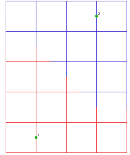
Consider following illustrative figure, there are two point features representing supply (e.g., hydrant locations). Some of the road line-strings are colored in red, and they are the portion of the network that is closest to point 1. The remaining road line-strings are colored in blue, meaning they are closest to point 2. This is a visualization of AdjFind road-segmentation mode’s result: a road line-string will be assigned to its closest service point (a.k.a. supply point), and the distance between each of its endpoint to the closest service point will be recorded in the attribute table (not shown here). If a road line-string has a portion closest to point 1 while the other portion closest to point 2, an equilibrium point (distance to either point is equal) along the line-string will be identified, and the original line-string will be split into two new line-strings; any point on the final output line-string is guaranteed to be closest to its assigned service point.

If we not only want to know the closest service point for each road line-string, but also want to know which portion of the network has a distance bracket/category 100–200 etc, it is also possible via road-segmentation mode with distance-breakpoints parameter.

In the above illustrative figure, I set distance-breakpoints parameter to 100,200,300, which implies 4 distance brackets: 0–100 (green), 100–200 (yellow), 200–300 (red), and ≥300 (purple). The algorithm performs further splitting on road line-strings in addition to the previous example; that is, if a road line-string has a point with distance to closest supply location the same as any of the breakpoint values, it will be split to two new line-strings at that breakpoint distance. Any point on the final output line-string except the endpoint is guaranteed to belong to one and only one distinct distance bracket.

What advantages does this road segmentation tool offer then?

• Demand may distribute continuously along the road line-strings, and this tool performs segmentations on road line-strings instead of requiring user to create discrete demand points for network-based analysis
• Euclidean distance fails to take road network into account and thus can be inaccurate, and this tool is network-distance based
• Traditional isochrone or service area analysis only tells coverage (an if question) but not true proximity (distance value), but this tool can tell the access distances to the line-string endpoints as well as line-string-level distance bracket
• Isochrone or service area analysis can generate concentric service areas (multiple breakpoints). This tool also gives user control with possibility of specifying multiple distance breakpoints. Additionally, the ability of this tool to tell the closest supply/service point is not restricted by any threshold or cutoff value.

In this article, I will also detail how AdjFind road segmentation algorithm works.

Constructing graph with points snapped

The first step is to read the input road line-string dataset. A line-string consists of two or more points, and it may consist of one or more consecutive segments; a segment is just a pair of points. This distinction is important. Each record in the input dataset is expected to be a line-string, but boost geometry only supports r-tree creation for segment but not line-string. Therefore, I initialize an vector for storing road line-strings, and the road r-tree is created such that each segment has corresponding line-string vector position index as well as the segment index for that particular line-string.

The second step is to read the input point dataset and “snap” each point to closest road line-string. This involves querying the road r-tree to obtain the (Euclidean-distance) closest road line-string, the segment index, and the closest point on the segment by projecting the point to the segment. The snapping information is stored as an unordered map, with road line-string index as key and a vector of the snapped point information as value; this setup addresses the possibility that multiple points are snapped to the same road line-string feature.

The third step is to create the graph. A graph consists of a set of vertices as well as edges connecting vertices. I use a point r-tree to store graph vertices, and a new vertex will be created if it is not within a distance tolerance threshold (assumed to be 0.01) from any existing vertex. Multiple edges with the same from vertex and to vertex can exist in the graph. To start the graph construction, I loop through the unordered map containing the snapping information. Within the loop, the road line-string will be marked as deleted (i.e., soft delete) since at least one point is snapped to it and its geometry will be replaced by new line-strings. The vector of snapped points will be sorted by segment index first, and the distance between the start of the segment and the snapped point second. Then I have an inner loop to iterate through the sorted snapped points to construct new line-strings with the snapped points taking into account; the new line-strings will be added as edges to the graph (when an edge is created, the corresponding vertices will either be from existing vertices or creating new ones). After looping through the unordered map, all the road line-strings that are not marked as deleted will be added as edges to the graph.

Populating closest point vertex for all intersection vertex

When constructing the graph, there are two types of vertices: one is intersection vertex (the input line-strings’ start and end points) and one is point vertex (the locations along the road line-strings where the supply points are snapped to). For any point vertex, its closest supply point is itself.

For all the intersection vertex though, a shortest path algorithm is needed to determine their closest point vertices. The shortest path algorithm used here is a variant of single-source Dijkstra algorithm. The source will the one of the intersection vertex. There is no fixed target; as soon as a point vertex is finalized/labeled, the path algorithm can stop searching. That finalized point vertex will correspond to the supply point that is closest to the source intersection vertex. In fact, any intermediate vertex traversed in the shortest path will have this same point vertex as its closest point vertex. In other words, after the shortest path is constructed, we can update all the traversed intersection vertices along the path (if the vertex is not updated yet) instead of just the source vertex; there is no need to run the path algorithm for every intersection vertex (but its closest point vertex is still determined by the path algorithm when using another intersection vertex as source).

Splitting a line-string at equilibrium point

After the previous steps, the closest point vertex as well as the corresponding distance are known for all vertices in the graph. If both vertices of an edge have the same closest point vertex, there is no need to split that edge. Otherwise, a portion of the edge is closest to one point vertex, while the other portion of the same edge is closest to another point vertex; a splitting step is necessary to ensure the output line-string (whose geometry sourced from the edge) uniquely closest to one point vertex.

The point on the edge where the split should occur should have the same network distance value to (i) edge’s from-vertex closest point, (ii) edge’s to-vertex closest point. We can setup a simple equation like following, where distance from the from-vertex is the unknown to solve:

from-vertex distance to closest point + distance from the from-vertex = to-vertex distance to closest point + (edge length - distance from the from-vertex)

The unknown can then be expressed with known variables:

distance from the from-vertex = 0.5 (to-vertex distance to closest point - from-vertex distance to closest point + edge length)*

With the distance measured from the edge’s from-vertex calculated by the above formula, it is possible to use boost geometry’s line_interpolate method to get the split point. The original edge entry will be updated with one of the new split edge, and a new edge entry will also be added to the edges vector.

Optionally splitting a line-string with distance breakpoints

The step described here is optional and only applies if distance-breakpoints parameter is set. If the parameter is not set (default), the edges from above step will be extracted and written as the output line-string dataset.

An edge has two vertices, and one of the vertices should be closer to the point vertex than the other vertex; this vertex that is closer to the point vertex, along with whether it is edge’s from-vertex or to-vertex, is stored as an attribute of the edge. The distance from the closest point vertex to this vertex is referred as distance_to_point_vertex here for simplicity.

In this step, there is an outer loop that iterates through each edge in the graph, and there is an inner loop that iterates through each element in the distance breakpoints vector. If the value obtained by subtracting a distance breakpoint value with the distance_to_point_vertex is non-negative and is smaller than edge length, it is necessary to interpolate along the edge with this value as the interpolation distance. The interpolated points will be used to construct output line-strings so that each output line-string can belong to one and only one distance bracket.

AdjFind is a C++ CLI program that you can install via homebrew tap (unfortunately the repo does not meet the popularity requirement of homebrew-core). If you like it, please star or fork the repo. Please also feel free to comment on this article with any question you have related to the algorithm, any bug reporting on GitHub Issues is very welcomed as well.

I am actively working on making it available via conda-forge; hopefully my PR gets approved.