Classification

A recap of Andrew Ng course (Machine Learning Specialization) on Coursera

Course 1 Week 3

Photo by Anusha Barwa on Unsplash

Motivations

ML practitioners set positive class for the phenomenon that they are interested in, so positive class doesn’t necessarily mean good class.

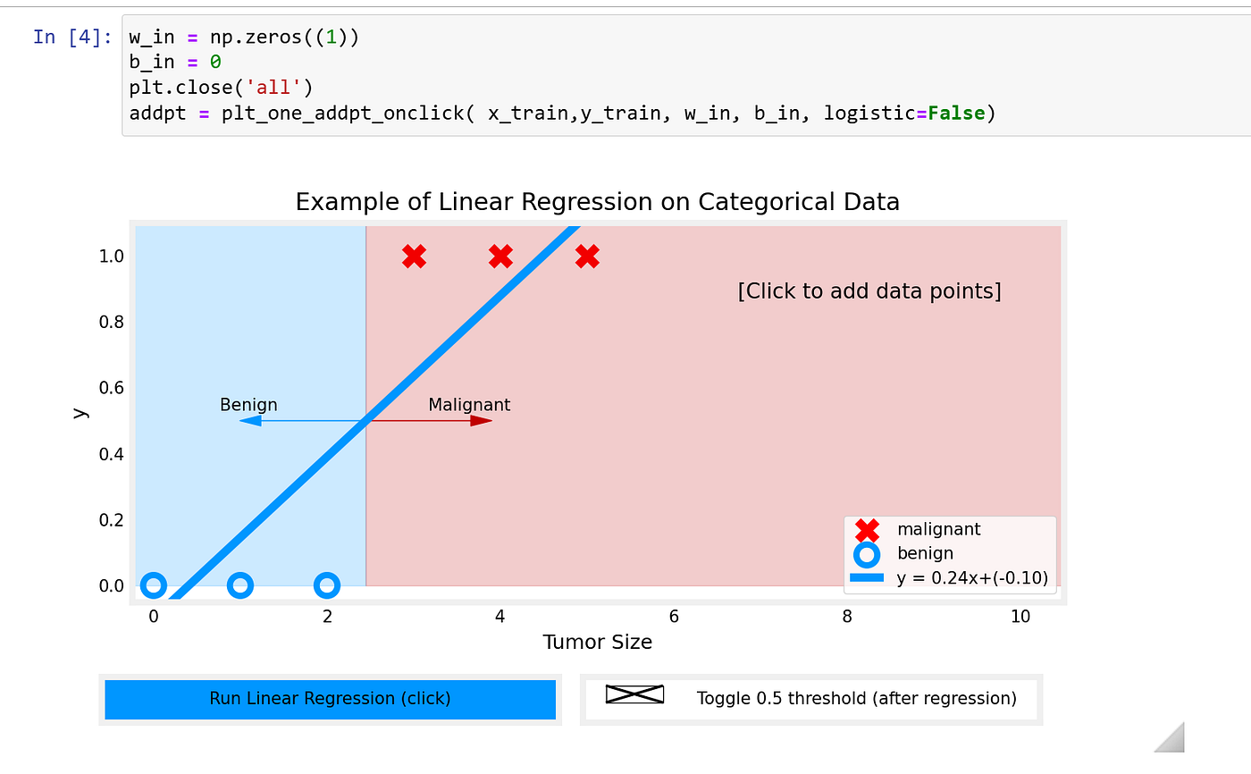
Linear regression is not sufficient to solve classification problems, because an outlier data point would affect the line created using linear regression. with a simple dataset as 3 negatives and 3 positives shown as below, we trained a linear regression to find a straight line to divide the negatives and positives, then we set a threshold like y = 0.5 as a classification boundary, it works ok for this dataset.

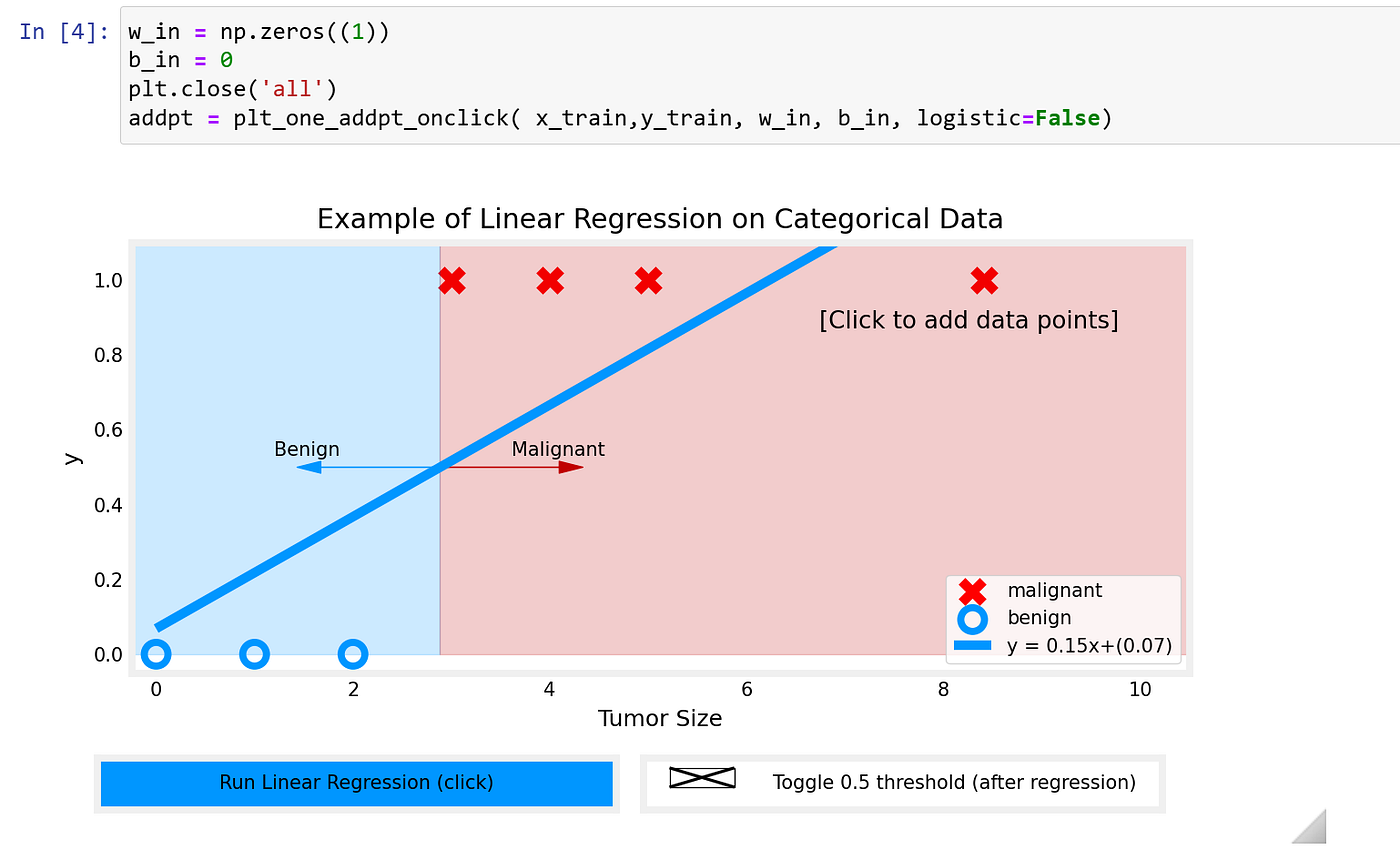
However, if we were to add a new data point, an outlier, to the malignant set, and then fit these 7 data points using linear regression again, we will see that the line was dragged further towards the outlier, and when we apply the y = 0.5 threshold now, x = 3 would be incorrectly classified as benign.

Logistic Regression

We need logistic regression to do classification since our label is 0 and 1. we need to learn a new function called sigmoid function a.k.a logistic function

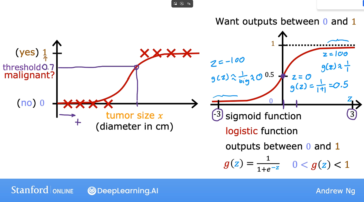
sigmoid function turns very large number close to 1 because e to the negative of a large number is close to 0; and this function turns very small number close to 0 because e to the negative of a very small number is a big number.

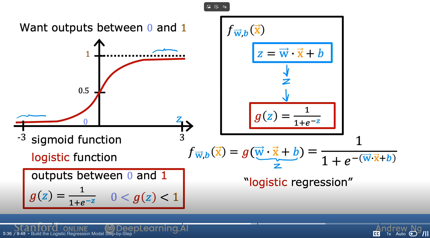
we combine the sigmoid function to the linear regression, and we get a logistic regression algorithm. the input to the sigmoid function is the output of a linear regression model.

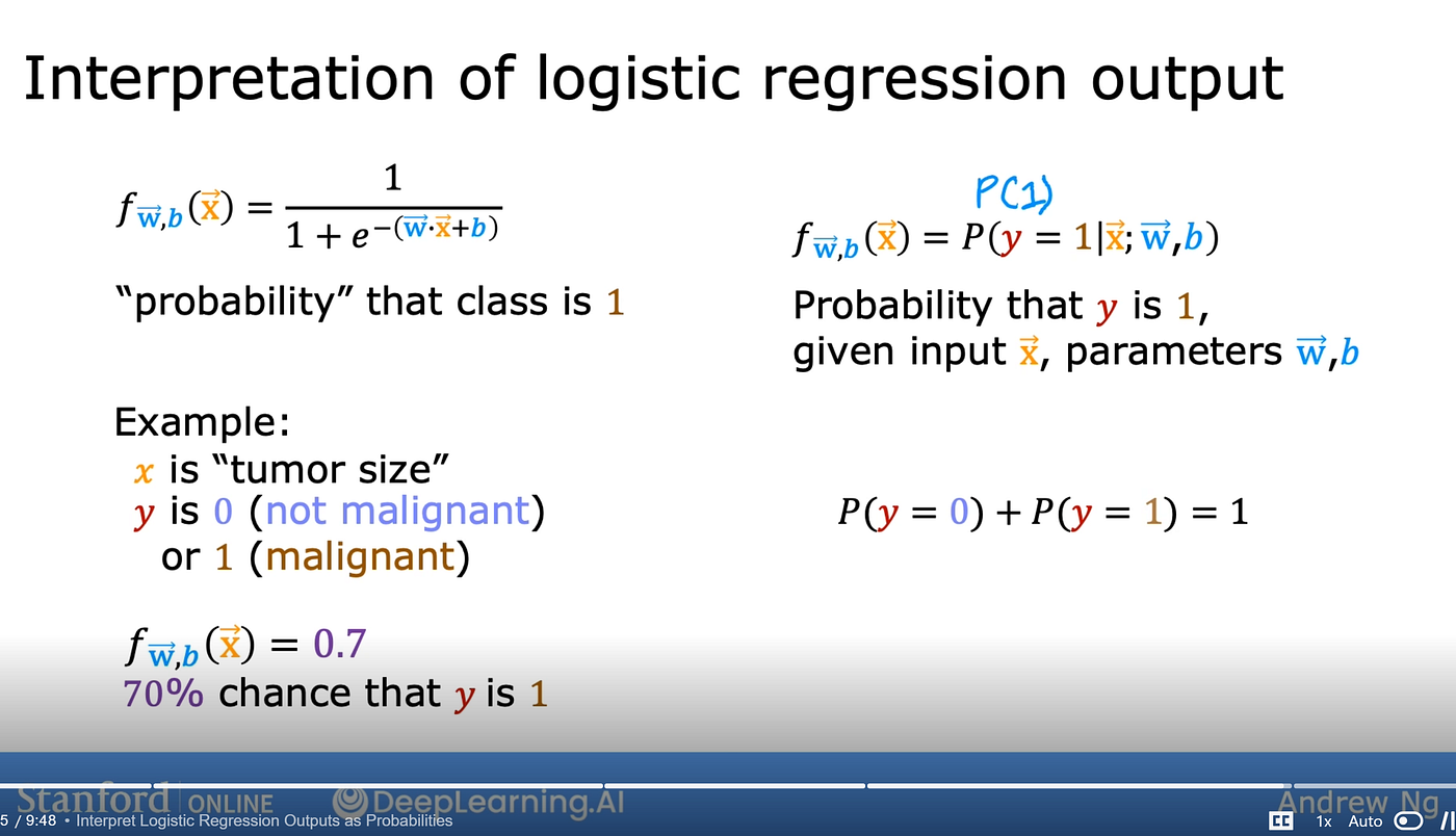
we can think of the logistic regression output as the probability that the class is Positive. So, if f(x) = 0.7, it means 70% chance that y is 1 and since there are only two classes, so the chance that y is 0 is 30%. some paper also writes logistic regression using P(y=1|x;w,b), probability that y is 1 given input x and parameters w and b.

Logistic regression and its variations have been very popular for some large websites when they do internet advertising for a long time

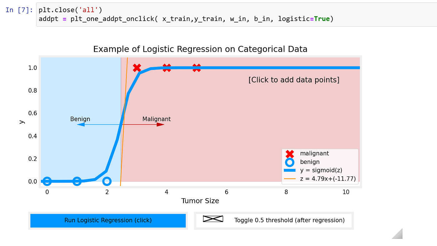
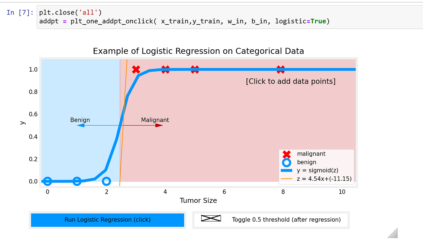
we do the same analysis again, and this time adding an outlier wouldn’t affect the results

Decision Boundary

right now, the output of sigmoid function is still not 0 and 1, the output is still a probability. we need to set a threshold above which we predict y as 1, and below which the pred is 0

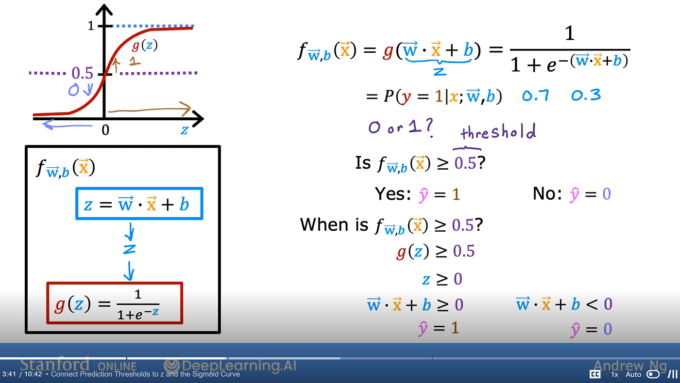
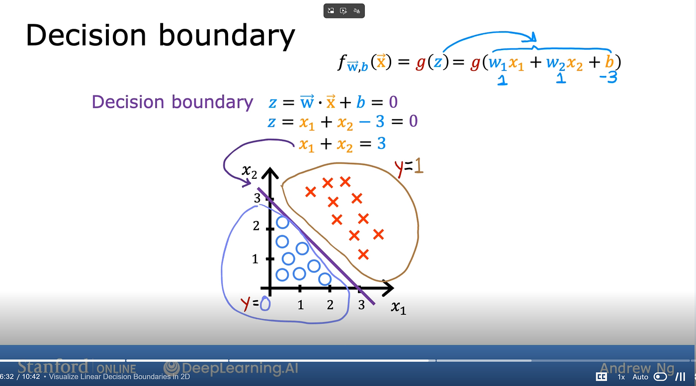
we use a threshold 0.5, namely, when the output of sigmoid function is greater than 0.5, we predict 1. g(z) ≥ 0.5 means z ≥ 0. so we can find when wx+b ≥ 0 to get positive outputs from the logistic regression model

we call the line wx+b = 0 the decision boundary for logistic regression, because that is the point when the line is almost neutral about positive or negative. we can visualize the decision boundary and set w1 = 1 and w2 = 1 and b = -3. so, the purple line is the decision boundary, every point to the left of it will be negative. if we set different values to w and b, we would get a different decision boundary

Non-linear decision boundary

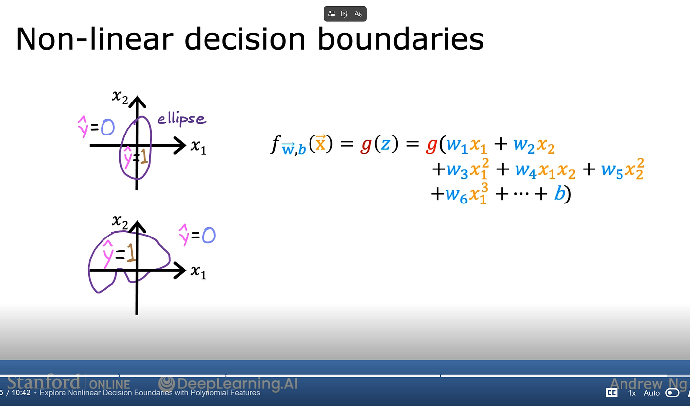
we saw how to use polynomial for linear regression, and we can also apply that to logistic regression

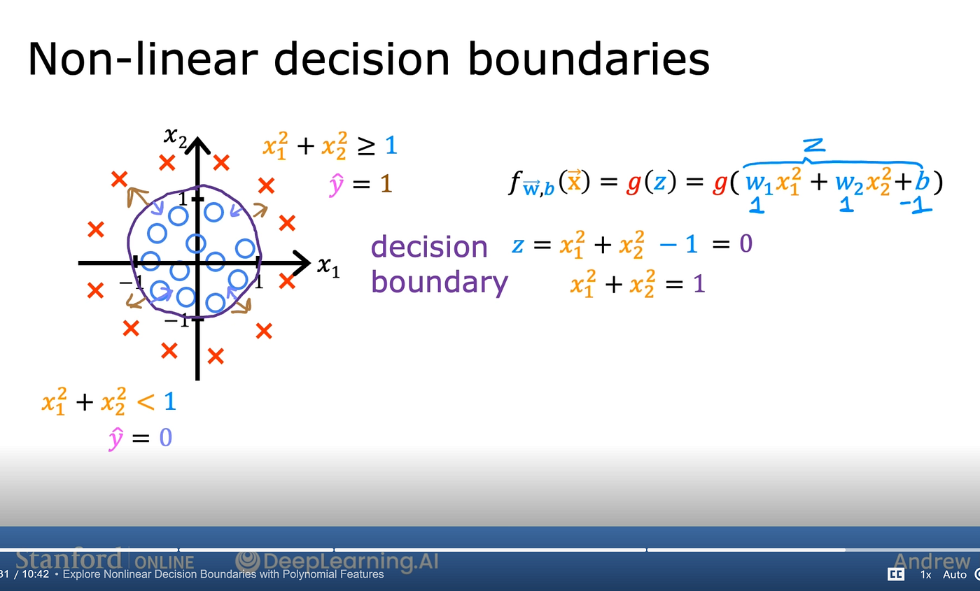
we can also create very complex data as below, in other words, logistic regression can be fit to very complex data. if we don’t use the squared features, then the logistic regression boundaries would always be linear, a straight line