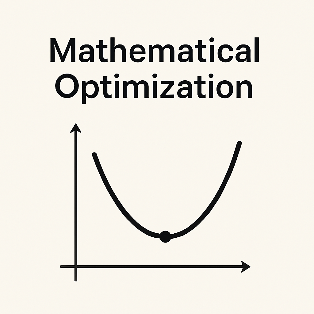
About Mathematical Optimization

• definition : finding an optimization variable that minimizes(or maximizes) an objective function

The birth

In An astronomy problem, scientists attempted to determine the trajectory of a celestial object based on 19 observations. However, recovering the exact trajectory was challenging.Gauss took an approach to estimate it, and his method laid the foundation of the optimization field.

Gauss’s approach

Gauss used 9 observations to predict the trajectory.

1. Fix two observed points.
2. Draw an orbit that passes through these two points. An orbit can be represented by six parameters.
3. To simplify, let x ∈ R⁴ denote the remaining unknown parameters.
4. Choose one additional point and compute the distance between the observed point and the predicted orbit. The relationship can be approximated as a linear model: A₁x ≈ b₁
5. Repeat this process for other observation points to obtain: Aᵢx ≈ bᵢ, i = 1, …, m
6. For the ground-truth orbit, each residual(|Aᵢx − bᵢ|) should be small.
7. Therefore, Gauss minimized the total squared error: minₓ ∑ |Aᵢx − bᵢ|²

This problem is known as the least-squares problem, which marked the beginning of the optimization field. It admits a closed-form solution:

x* = (AᵀA)⁻¹Aᵀb

and can be efficiently computed using numerical methods such as QR decomposition.

Afterward, many problems were reformulated as least-squares problems through various translation techniques.

Leonid Kantorovichi

During World War II, Leonid Kantorovich worked on a resource allocation problem related to the military. He formulated it as a linear programming (LP) problem. Although LPs generally have no closed-form solution, they can be solved efficiently with algorithms that guarantee the global optimum (e.g., the simplex or interior-point methods). He was awarded the 1975 Nobel Prize in Economic Sciences for this work. Many other real-world problems have since been translated into LPs.

From Tractable Problems to Convex Optimization

Tractable optimization problems such as least-squares and linear programs are special cases of convex optimization.

About Convex Optimization

A general convex optimization problem can be written as:

where

• x ∈ Rⁿ is the optimization variable,
• f(x) is the objective function,
• fᵢ(x) are inequality constraints, and
• hᵢ(x) are equality constraints.

The optimal solution is defined as:

x* = argminₓ f(x) subject to fᵢ(x) ≤ 0, hᵢ(x) = 0

and the corresponding optimal value is p = f(x).

If both the objective function f(x)and the feasible set defined by the constraints are convex, the problem is convex. For convex problems, efficient algorithms such as gradient descent or interior-point methods are guaranteed to find the global optimum.

Convex set

A set S ⊆ Rⁿ is said to be convex if and only if:

x, y ∈ S ⇒ λx + (1 − λ)y ∈ S, ∀ λ ∈ [0,1]

This property means that every line segment connecting two points in the set lies entirely within the set. Such combinations are called convex combinations.

Affine Function and Affine Set

An affine function is a linear function plus a translation: f(x) = A x + b

An affine set is any set closed under affine combinations:

x, y ∈ S ⇒ λx + (1 − λ)y ∈ S, ∀ λ ∈ R with λ + (1 − λ) = 1

Equivalently, an affine set can be described as the solution set of a system of linear equations:

S = { x ∈ Rⁿ | Fx = g }

Affine sets are always convex, and affine functions preserve convexity.

Polygon, Polyhedra and Polytopes

A polyhedron is the intersection of finitely many closed half-spaces:

P = { x ∈ Rⁿ | Ax ≤ b }

A polytope is a bounded polyhedron, equivalently defined as the convex hull of finitely many points:

P = conv{v₁, v₂, …, vₖ}

In two dimensions, a closed polygon is a simple example of a polytope.

Convex Function

A real-valued function f(x) is said to be convex if

x, y ∈ dom f, ∀ λ ∈ [0,1]:f(λx + (1 − λ)y) ≤ λf(x) + (1 − λ)f(y)

Here, dom f must be a convex set. Intuitively, convex functions are “bowl-shaped.” Affine functions are both convex and concave.

Real-world deep learning problems

Real-world deep learning problems are typically highly non-convex and therefore intractable in theory — there is no guarantee of finding a global optimum. Still, method for solving convex opt are often powerful for DL(ex. Gradient Descent)