Detecting Green Cells in Grid Squares: A Step-by-Step Guide with OpenCV and Python (Part 2)

In previous post, I updated code with features includes:

1. Loading and converting the image to grayscale.
2. Detecting edges in the grayscale image.
3. Detecting lines using the Hough Line Transform.
4. Merging nearby lines to reduce redundancy.
5. Indexing each square in the image.

Previous post: https://medium.com/@shiodev/analyzing-and-processing-grid-images-with-opencv-part-1-d5c42ab0703c

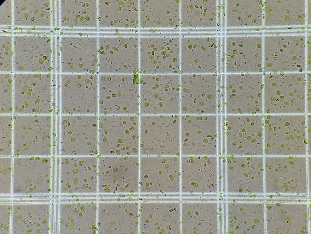
In this post, I will create a function to crop each square into multiple images. This will be useful for the subsequent procedure of counting the number of plant cells in each square area.

Step 6: Index and Crop the Squares (Updated)

Finally, we index each square in the image, crop them, and save the cropped squares as separate images.

def index_and_crop_squares(image, horizontal_lines, vertical_lines):
    index = 1
    horizontal_lines_excluding_top = horizontal_lines[1:]
    cropped_squares = []

    for i in range(len(horizontal_lines_excluding_top) - 1):
        for j in range(len(vertical_lines) - 1):
            top_left = (vertical_lines[j], horizontal_lines_excluding_top[i])
            bottom_right = (vertical_lines[j + 1], horizontal_lines_excluding_top[i + 1])
            # Crop the square
            cropped_square = image[top_left[1]:bottom_right[1], top_left[0]:bottom_right[0]]
            cropped_squares.append((index, cropped_square))
            index += 1
    return cropped_squares

def process_image_and_save_squares(image_path, num_squares=5):
    image, gray_image = load_and_convert_image(image_path)
    edges = detect_edges(gray_image)
    lines = detect_lines(edges)
    _, merged_horizontal_lines, merged_vertical_lines = merge_nearest_lines(lines, image)
    cropped_squares = index_and_crop_squares(image, merged_horizontal_lines, merged_vertical_lines)

    saved_squares = []
    for i in range(min(num_squares, len(cropped_squares))):
        square_index, square_image = cropped_squares[i]
        square_path = f'./processing_data/square_{square_index}.jpg'
        cv2.imwrite(square_path, square_image)
        saved_squares.append(square_path)

    return saved_squares

# Usage example
image_path = 'path_to_your_image.jpg'
saved_square_paths = process_image_and_save_squares(image_path, num_squares=5)

Result:

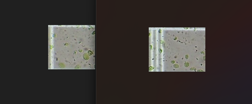
Cropped square image

Step 7: Detect Green Cells And Improve Function

We will now add a function to detect green cells in the image.

Result from test function:

import cv2
import numpy as np
import matplotlib.pyplot as plt

# Load the image
image_path = './processing_data/square_1.jpg'
image = cv2.imread(image_path)

# Convert the image to HSV color space
hsv_image = cv2.cvtColor(image, cv2.COLOR_BGR2HSV)

# Define the range for green color in HSV
lower_green = np.array([40, 40, 40])
upper_green = np.array([80, 255, 255])

# Create a mask for the green color
mask = cv2.inRange(hsv_image, lower_green, upper_green)

# Find contours in the mask
contours, _ = cv2.findContours(mask, cv2.RETR_EXTERNAL, cv2.CHAIN_APPROX_SIMPLE)

# Count the number of green cells
number_of_green_cells = len(contours)

# Draw contours on the original image
output_image = image.copy()
cv2.drawContours(output_image, contours, -1, (0, 255, 0), 2)

# Display the result
plt.figure(figsize=(10, 10))
plt.subplot(1, 2, 1)
plt.title('Original Image')
plt.imshow(cv2.cvtColor(image, cv2.COLOR_BGR2RGB))
plt.subplot(1, 2, 2)
plt.title('Green Cells Counted')
plt.imshow(cv2.cvtColor(output_image, cv2.COLOR_BGR2RGB))
plt.show()

Do the function to detect the green cell

Result:

25

It still have a lot of noise here. So I continue adjust the HSV value again.

Green plant cells typically have a distinct green color due to chlorophyll, which can be effectively detected in the HSV color space. The HSV range for green typically falls within these ranges:

• Hue (H): 35 to 85
• Saturation (S): 40 to 255
• Value (V): 40 to 255

def detect_green_cells(image_path, min_area_threshold=100, display_result=True):
    # Load the image
    image = cv2.imread(image_path)

    # Convert the image to HSV color space
    hsv_image = cv2.cvtColor(image, cv2.COLOR_BGR2HSV)

    # Define the HSV range for green color detection
    lower_green = np.array([30, 30, 30])
    upper_green = np.array([90, 255, 255])

    # Create a mask for the green color
    mask_green = cv2.inRange(hsv_image, lower_green, upper_green)

    # Apply morphological transformations to remove noise and better define the cell boundaries
    kernel = np.ones((3, 3), np.uint8)
    mask_green_morphed = cv2.morphologyEx(mask_green, cv2.MORPH_CLOSE, kernel)
    mask_green_morphed = cv2.morphologyEx(mask_green_morphed, cv2.MORPH_OPEN, kernel)

    # Find contours in the morphed mask
    contours, _ = cv2.findContours(mask_green_morphed, cv2.RETR_EXTERNAL, cv2.CHAIN_APPROX_SIMPLE)

    # Filter contours by area
    filtered_contours = [cnt for cnt in contours if cv2.contourArea(cnt) > min_area_threshold]

    # Draw filtered contours and bounding boxes on the original image
    output_image = image.copy()
    for cnt in filtered_contours:
        x, y, w, h = cv2.boundingRect(cnt)
        cv2.drawContours(output_image, [cnt], -1, (0, 255, 0), 2)
        cv2.rectangle(output_image, (x, y), (x + w, y + h), (255, 0, 0), 2)
        area = cv2.contourArea(cnt)
        cv2.putText(output_image, f'Area: {area}', (x, y - 10), cv2.FONT_HERSHEY_SIMPLEX, 0.5, (255, 0, 0), 1)

    # Display the result if requested
    if display_result:
        plt.figure(figsize=(10, 10))
        plt.title('Green Cells Detection')
        plt.imshow(cv2.cvtColor(output_image, cv2.COLOR_BGR2RGB))
        plt.show()

    # Return the number of detected cells and the output image with annotations
    return len(filtered_contours), output_image

# Example usage
image_path = './processing_data/square_1.jpg'
num_cells, annotated_image = detect_green_cells(image_path)
print(f"Number of green cells detected: {num_cells}")

Test with square_1.jpg. The detection process for the new image identified 8 cell detected while I can see ~10–11 cells.

Test with square_2.jpg. The detection process for the new image identified 12 green cells while I can identify about 13–14 cells.

Summary

The presented method demonstrates a robust approach to detecting and analyzing plant cells in microscopic images using OpenCV. This technique can be further refined and adapted for other types of cells or imaging conditions. The combination of color-based segmentation and morphological processing proves effective in isolating and quantifying plant cells, aiding in various research endeavors.

Future Work

Future improvements could include:

• Implementing machine learning models for more adaptive color segmentation.
• Enhancing image resolution and clarity to improve detection accuracy.
• Applying the methodology to other cell types and imaging modalities.

Enjoy!

Katanuki