The Central Limit Theorem: Why the Normal Distribution Rules the World

Part 2 of a series on the two pillars of probability theory.

Introduction

If the Law of Large Numbers (covered in Part 1) tells us where an average is going, the Central Limit Theorem tells us how it gets there. It is arguably the single most consequential result in all of statistics — the reason the bell curve appears in test scores, measurement errors, financial returns, polling margins, and quality control charts. The Central Limit Theorem (CLT) explains a minor miracle: no matter how strange, skewed, or lumpy a population is, the distribution of sample means drawn from it converges toward a normal distribution as the sample size grows.

The Core Idea, Stated Plainly

Let there be a population with a finite mean μ and finite variance σ². The population itself may have any shape — uniform, exponential, bimodal, wildly skewed. Suppose samples of size n are drawn repeatedly from this population, and the mean of each sample is computed.

The Central Limit Theorem makes three claims about the distribution of those sample means:

1. Its shape approaches a normal distribution as n increases, regardless of the population’s shape.
2. Its center equals the population mean: E[X̄] = μ.
3. Its spread shrinks predictably: SD(X̄) = σ/√n, a quantity known as the standard error.

The third point deserves emphasis. The √n in the denominator implies that halving the uncertainty in an estimate requires quadrupling the sample size. This law of diminishing returns governs the economics of every survey, clinical trial, and A/B test ever conducted.

The Formal Statement

Let X₁, X₂, …, Xₙ be independent and identically distributed (i.i.d.) random variables with E[Xᵢ] = μ and Var(Xᵢ) = σ² < ∞. The sample mean is defined as:

X̄ₙ = (1/n) Σ Xᵢ

The Central Limit Theorem states that the standardized sample mean converges in distribution to the standard normal:

√n (X̄ₙ − μ) / σ → N(0, 1) as n → ∞

Equivalently, for large n, the sample mean is approximately distributed as:

X̄ₙ ≈ N(μ, σ²/n)

Two technical points merit attention. First, the convergence is in distribution — a statement about the shape of probabilities, weaker than the almost-sure convergence of the Law of Large Numbers. Second, the only requirements are independence, identical distribution, and finite variance. Nothing about the population needs to be normal. Therein lies the entire magic of the theorem.

A Sketch of Why It Works

A full proof employs characteristic functions (the Fourier transform of a distribution). The essence is as follows: the characteristic function of a sum of independent variables is the product of their individual characteristic functions. When the sum is standardized, and each characteristic function is expanded as a Taylor series, the first-order terms vanish (centering removes the mean), the second-order terms accumulate into exp(−t²/2) — precisely the characteristic function of the standard normal — and all higher-order terms are crushed by the √n scaling. The idiosyncrasies of the original distribution reside in those higher-order terms, and they die as n grows. Only the mean and variance survive the limit.

Seeing It in Python

Theory becomes conviction through simulation. The code below draws samples from an exponential distribution — a heavily right-skewed population that looks nothing like a bell curve — and tracks how the sample means organize themselves into a normal distribution.

import numpy as np
import matplotlib.pyplot as plt
from scipy import stats

np.random.seed(42)

# A deliberately non-normal population: exponential with mean 1
population_mean = 1.0
population_std = 1.0   # for Exp(1), mean = std = 1

sample_sizes = [1, 5, 30, 100]
n_simulations = 10_000

fig, axes = plt.subplots(1, 4, figsize=(18, 4))

for ax, n in zip(axes, sample_sizes):
    # Draw 10,000 samples of size n; compute each sample's mean
    sample_means = np.random.exponential(scale=1.0,
                                         size=(n_simulations, n)).mean(axis=1)

    print(f"n = {n:3d} | mean of sample means = {sample_means.mean():.4f} | "
          f"SD = {sample_means.std():.4f} | "
          f"theory σ/√n = {1/np.sqrt(n):.4f} | "
          f"skew = {stats.skew(sample_means):+.3f}")

    ax.hist(sample_means, bins=60, density=True,
            color="steelblue", alpha=0.7, edgecolor="white")

    # Overlay the normal curve predicted by the CLT
    x = np.linspace(sample_means.min(), sample_means.max(), 300)
    se = population_std / np.sqrt(n)
    normal_pdf = (1 / (se * np.sqrt(2 * np.pi))) * \
                 np.exp(-0.5 * ((x - population_mean) / se) ** 2)
    ax.plot(x, normal_pdf, "r-", lw=2, label="CLT prediction")

    ax.set_title(f"n = {n}\nSE = {se:.3f}")
    ax.legend()

plt.suptitle("Sample means of an Exponential(1) population", fontsize=14)
plt.tight_layout()
plt.show()

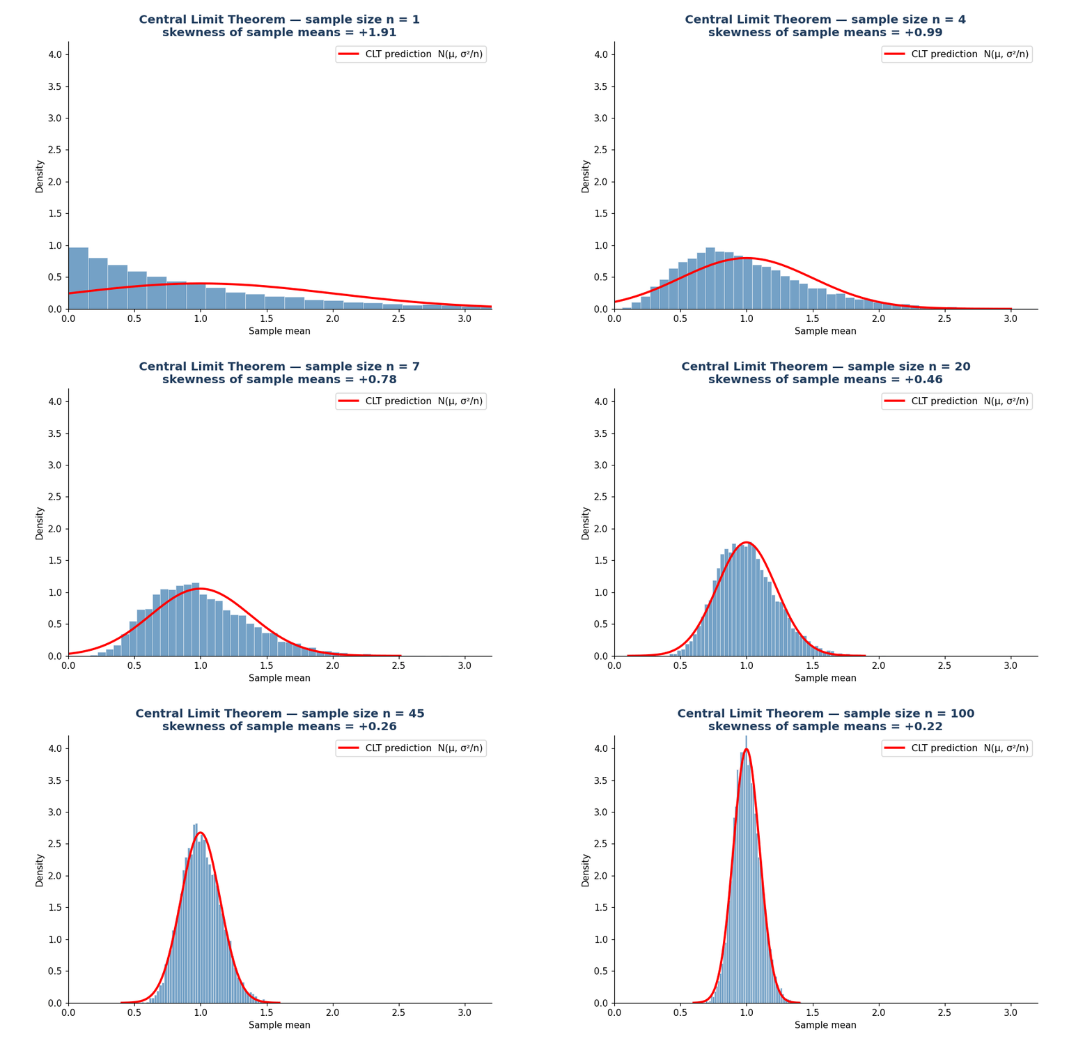
four-panel histograms at n = 1, 5, 30, 100 with red CLT prediction curves

![formatted output table — mean of sample means, SD, theory σ/√n, skewness]](https://miro.medium.com/v2/resize:fit:1400/1*QdZi7vHbEa_57aRWj9mktg.png)

formatted output table — mean of sample means, SD, theory σ/√n, skewness]

The numbers tell the whole story before the plots do. At every sample size, the mean of the sample means sits at the population mean of 1; that is claim (2). The empirical standard deviation of the sample means tracks the theoretical σ/√n to two or three decimal places; claim (3): 0.4480 versus 0.4472 at n = 5, and 0.1009 versus 0.1000 at n = 100. Meanwhile, the skewness, the fingerprint of the exponential’s asymmetry, collapses from +1.92 (essentially the raw population, since n = 1) to +0.17 at n = 100. That is claim (1) in action: the population’s shape being averaged out of existence.

The visual progression is equally striking. At n = 1, the histogram simply reproduces the skewed exponential shape. At n = 5, a hump begins to form, but the right tail lingers. By n = 30, the folk threshold quoted in every introductory course, the histogram is nearly indistinguishable from the red normal curve. At n = 100, the agreement is essentially perfect.

Quantifying the Convergence

The analysis can go beyond visual inspection: the discrepancy between the sample-mean distribution and the normal distribution can be measured directly.

from scipy import stats

for n in [2, 5, 10, 30, 100, 500]:
    sample_means = np.random.exponential(1.0, size=(10_000, n)).mean(axis=1)
    # Standardize using the CLT's predicted mean and standard error
    z = (sample_means - 1.0) / (1.0 / np.sqrt(n))
    # Kolmogorov–Smirnov distance to the standard normal
    ks_stat, _ = stats.kstest(z, "norm")
    print(f"n = {n:4d}  |  skew = {stats.skew(sample_means):+.3f}"
          f"  |  KS distance = {ks_stat:.4f}")

formatted table — skewness and KS distance for n = 2 to 500

The Kolmogorov–Smirnov distance — the largest gap between the empirical distribution of standardized sample means and the true standard normal — shrinks monotonically, roughly halving each time n grows by a factor of four or five. This is no accident: the Berry–Esseen theorem guarantees that the error decays at rate C/√n, giving the CLT not merely a promise of convergence but a speed limit on it. The KS distance drops from 0.0911 at n = 2 to 0.0167 at n = 100 — a more than fivefold improvement, of the same order as the √50 ≈ 7× reduction the theorem predicts.

Log-log plot of empirical KS distance against the Berry–Esseen 1/√n rate line

Worked Example: The Insurance Company’s Dilemma

Abstract theorems earn their keep through concrete decisions. An instructive case is an insurer covering 10,000 policyholders. Each claim is wildly unpredictable — most policyholders claim little or nothing in a year, while a few claim enormous amounts. The simulation below models claims with a lognormal distribution tuned to a mean of approximately $500 per policyholder:

import numpy as np
from scipy import stats

np.random.seed(42)

# 2,000 simulated years, 10,000 policyholders each
claims = np.random.lognormal(mean=4.595, sigma=1.8, size=(2_000, 10_000))
totals = claims.sum(axis=1)

print(f"Individual claim: mean = {claims.mean():,.0f}, "
      f"SD = {claims.std():,.0f}, skew = {stats.skew(claims.ravel()):+.1f}")
print(f"Average claim per policyholder: mean = {claims.mean(axis=1).mean():.2f}, "
      f"SD = {claims.mean(axis=1).std():.2f}")
print(f"Theory SE = σ/√n = {claims.std()/np.sqrt(10_000):.2f}")
print(f"Total payout: mean = {totals.mean():,.0f}, SD = {totals.std():,.0f}")

formatted table — individual claim stats, average claim stats, theory SE, total payout stats

The contrast in that output is remarkable. A single claim has a skewness of +69.6 — a distribution so violently asymmetric that its standard deviation ($2,444) is nearly five times its mean ($500). Individually, these claims are close to unforecastable. Yet the average claim across 10,000 policies has a standard deviation of just $24.33, matching the CLT’s prediction of σ/√n = 2444/√10000 = $24.44 almost exactly.

violently skewed single-claim distribution on the left, bell-shaped total payout with normal fit on the right

The total payout is therefore approximately normal, with a mean of $5.0 million and a standard deviation of about $243,000. The insurer can set aside the mean plus three standard errors — roughly $5.73 million in reserves — and expect solvency in about 99.9% of years. An entire industry is built on this arithmetic: individual chaos, aggregated, becomes collective predictability.

Why the CLT Matters So Much

It is the engine of statistical inference. Every confidence interval of the form “estimate ± 1.96 × standard error” is a direct application of the CLT. Every z-test and, with a finite-sample correction, every t-test rests on the sample mean being approximately normal. Without the CLT, statistical inference would require knowing the exact population distribution in advance — which is precisely what is never known in practice.

It explains why the normal distribution is everywhere. Heights, measurement errors, and manufacturing tolerances tend toward normality because each is the sum of many small independent influences — genes, environmental factors, micro-vibrations. The CLT is nature’s averaging mechanism. Wherever many small independent effects add up, a bell curve emerges.

It justifies A/B testing and polling. When a pollster reports a “margin of error of ±3%,” that figure is 1.96 × √(p(1−p)/n) — the CLT applied to a Bernoulli population. When a product team declares an experiment significant, the underlying z-statistic assumes the CLT has already done its work on the conversion-rate averages.

It underlies machine learning practice. Mini-batch gradient estimates in stochastic gradient descent are sample means; their approximately normal fluctuation around the true gradient is a CLT phenomenon, and it shapes how learning rates and batch sizes trade off against one another.

Where the Theorem Breaks

Intellectual honesty requires stating the boundaries. The CLT fails, or slows dramatically, when its assumptions are violated.

Infinite variance. The Cauchy distribution has no defined mean or variance; averages of Cauchy variables are themselves Cauchy — no convergence ever occurs. Heavy-tailed phenomena such as financial crashes and city sizes can behave similarly, which is why naive normal approximations in risk management have caused genuine disasters.

Strong dependence. The i.i.d. assumption matters. Highly correlated observations (time series, clustered data) effectively shrink the sample size, and the standard error σ/√n becomes optimistically small. Generalized versions of the CLT exist for weakly dependent data, but the practitioner must know which regime applies.

Small n with extreme skew. “n ≥ 30” is a heuristic, not a law. As the tables above demonstrate, even at n = 30 the sample means retained a skewness of roughly +0.4 — visible asymmetry. For a distribution as extreme as the insurance claims (skew +69.6), convergence at small n would be far slower still. Simulation, as demonstrated throughout this article, is the honest way to check.

Conclusion

The Central Limit Theorem is the bridge between the unknowable and the estimable. The Law of Large Numbers promises that averages settle down; the CLT specifies the exact probabilistic law governing their fluctuations — normal, centered at μ, with spread σ/√n. That single formula converts raw data into confidence intervals, p-values, error margins, and risk reserves.

It is worth pausing on how remarkable the claim is: an infinite diversity of populations, all funneled by averaging into one universal shape. The normal distribution is not an assumption statisticians impose on the world. It is a destination the world arrives at on its own, wherever independence and aggregation are present. Understanding the CLT is understanding why statistics works at all.

For readers who wish to see these two pillars put to work making decisions under uncertainty, hypothesis testing has been covered in detail in two earlier articles by the author:

1. Statistical Hypothesis Testing Part I — The One-Tailed Test

2. Statistical Hypothesis Testing Part II — The Two-Tailed Test.

Every z-statistic and p-value in those articles rests on the theorem developed here.