Tropomi netCDF File Data to Raster Images Using a Moving Window Algorithm

Processing SRON RemoTeC-S5P XCH4 (for data click ***here***)

The netCDF files in the provided link contain data from the Sentinel-5P TROPOMI instrument. These files are organized by orbit and contain multiple types of data. Our goal is to gather this data and organize the polygons into 32x32 grids for processing.

Data storing and initial organization

import numpy as np
from netCDF4 import Dataset
import matplotlib.pyplot as plt
import matplotlib.colors as mcolors
from matplotlib.patches import Polygon
from matplotlib import colormaps
from mpl_toolkits.basemap import Basemap
import matplotlib.colors as mcolors
from matplotlib.colors import ListedColormap

nc = Dataset("H:\\18_17\\s5p_l2_ch4_0017_18985.nc", 'r')
"""
Storing data of interest into variables methane concentration,
polygons coordinates, wind, and others.
"""
#methane concentration xch4_corrected as recomemded by SRON
methane = nc.groups ['target_product'][ 'xch4_corrected'][:]

#wind data
u10 = nc.groups['meteo']['u10'][:]
v10 = nc.groups['meteo']['v10'][:]

#These are the polygon corners
latitude_corners = nc.groups ['instrument'][ 'latitude_corners'][:]
longitude_corners = nc.groups ['instrument'][ 'longitude_corners'][:]

#These are used to organize the data later on
ground_pixel_no_filter = nc.groups ['instrument'][ 'ground_pixel'][:]
scan_line_no_filer = nc.groups ['instrument']['scanline'][:]

"""
These are variables that will be used in 
the filtering of the dataset. 
"""

qa_value = nc.groups['diagnostics']['qa_value'][:]
precision = nc.groups['target_product']['xch4_precision'][:] 
surface_albedo = nc.groups['side_product']['surface_albedo'][:] 
cloud_fraction = nc.groups['meteo']['cloud_fraction'][:] 
aerosol_optical_depth= nc.groups['side_product']['aerosol_optical_thickness'][:]
relative_azimuth_angle = nc.groups ['instrument'][ 'relative_azimuth_angle'][:]
pixel_id_no_filter = nc.groups ['instrument'][ 'pixel_id'][:]

#center coordinate for each pixel 
#latitude_center = nc.groups ['instrument'][ 'latitude_center'][:]
#longitude_center = nc.groups ['instrument'][ 'longitude_center'][:]

#This is to get rid of indeces in the data set that dont correspond to any data.
non_masked_indices = np.where(~pixel_id_no_filter)[0]

# Extracting SWIR and NIR aerosol optical depths
nir_aerosol_optical_depth = aerosol_optical_depth[:, 0]  # first column
swir_aerosol_optical_depth = aerosol_optical_depth[:, 1]   # second column

#Extracting SWIR and NIR surface albedo
nir_surface_albedo = surface_albedo[:, 0]
swir_surface_albedo = surface_albedo[:,1]

# Mixed Albedo
mixed_albedo = 2.4*nir_surface_albedo[non_masked_indices]
               -1.13*swir_surface_albedo[non_masked_indices]

"""
SRON RemoTeC-S5P XCH4 product has given recomendations
for the parameters used in the filtering. Though I choose to
use the parameters that were described in the research paper. 
"""

filtered_indices = non_masked_indices[
    (qa_value[non_masked_indices] >= 0.4) &
    (precision[non_masked_indices] < 10) &
    (swir_aerosol_optical_depth[non_masked_indices] < 0.13) &
    (nir_aerosol_optical_depth[non_masked_indices] <0.30) &
    (swir_surface_albedo[non_masked_indices] > 0.02) &
    (mixed_albedo < 0.95) &
    (cloud_fraction[non_masked_indices][:,0] <0.02)
] 

#Apply the above filtering to the data
ch4 = methane[filtered_indices]
lat_corners = latitude_corners[filtered_indices]
lon_corners = longitude_corners[filtered_indices]
u_wind = u10[filtered_indices]
v_wind = v10[filtered_indices]
pixel_id = pixel_id_no_filter[filtered_indices]
ground_pixel = ground_pixel_no_filter[filtered_indices]
scan_line = scan_line_no_filer[filtered_indices]

#close the file
nc.close()

We can use data such as latitude_corners and longitude_corners to plot the polygons and the corresponding methane values for those polygons.

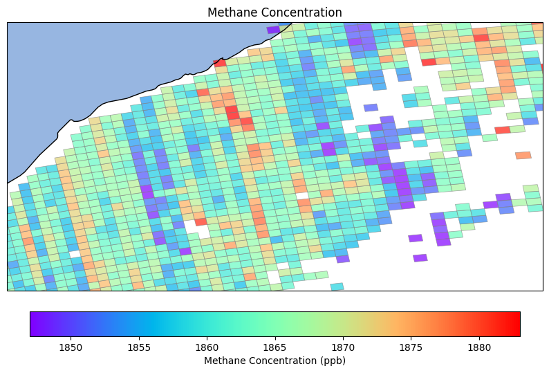
Plot example

To store the data in preparation for generating 32x32 pixel scenes, where we can store multiple variables per pixel, we use the scan_line and ground_pixel variables from the dataset. Below is a visualization of the scan lines and ground pixels.

Imagine each scan line as an array where the ground pixels define the index and the number of indices in that array.

# Define the dtype for the structured array
# Here we can add more forms of data that we want to contain in our scenes

dtype = [('ch4', 'f4'), ('lat_corners', 'f4', (4,)),('lon_corners','f4',(4,))] 

# Calculate the number of unique scan lines and ground pixels
max_scan_line = max(scan_line)
min_scan_line = min(scan_line)
max_ground_pixel = max(ground_pixel)
min_ground_pixel = min(ground_pixel)
num_scan_lines = max_scan_line - min_scan_line + 1
num_ground_pixels = max_ground_pixel - min_ground_pixel + 1

# Initialize the structured array
scan_line_lists = np.full((num_scan_lines, num_ground_pixels),
                           np.nan, dtype=dtype)

# Populate the array
for idx in range(len(ch4)):
    scan_idx = scan_line[idx] - min_scan_line
    pixel_idx = ground_pixel[idx] - min_ground_pixel
    scan_line_lists[scan_idx, pixel_idx] = (ch4[idx], lat_corners[idx],
                                            lon_corners[idx])

Now that we have our scan line arrays stored with the data we want, we will iterate over them 32 rows and 32 columns at a time, maintaining a 50% overlap both vertically and horizontally. Any matrices that we generate that do not contain 20% or more valid pixels for methane will not be included.

# Initialize list to store 32x32 matrices
ch4_matrices = []

def create_matrices(scan_line_lists):
    num_scan_lines = len(scan_line_lists)
    max_indices = len(scan_line_lists[0])

    # Loop through the scan lines with 50% vertical overlap
    for start_row in range(0, num_scan_lines, 16):
        if start_row + 32 > num_scan_lines:
            break

        # Loop through the indices with 50% horizontal overlap
        for start_col in range(0, max_indices, 16):
            if start_col + 32 > max_indices:
                break

            # Create a 32x32 matrix of type object
            matrix = np.empty((32, 32), dtype=dtype)
            for i in range(32):
                if start_row + i < num_scan_lines:
                    row_data = scan_line_lists[start_row + i]
                    for j in range(32):
                        if start_col + j < max_indices:
                            # Store a tuple of ch4 and lat_corners
                            ch4_value = row_data[start_col + j]['ch4']
                            lat_corners_value = row_data[start_col + j]['lat_corners']
                            lon_corners_value = row_data[start_col + j]['lon_corners']
                            matrix[i, j] = (ch4_value, lat_corners_value, lon_corners_value)

            # Only append the matrix if it has 20% or more non-NaN values
            if np.count_nonzero(~np.isnan(matrix['ch4'])) > 204:
                ch4_matrices.append(matrix)

# Create the matrices
create_matrices(scan_line_lists)

This function was used to apply the normalization of the data for each matrix.

def normalize_matrix(matrix):
    mean_ch4 = np.nanmean(matrix)
    std_ch4 = np.nanstd(matrix)
    lower_bound = mean_ch4 - std_ch4
    upper_bound = mean_ch4 + 100 - std_ch4  # 100 ppb added to mean, then subtract std
    #print(mean_ch4, std_ch4, lower_bound, upper_bound)
    # Replace NaN values with 0

    matrix = np.where(np.isnan(matrix), 0, matrix)
    # Normalize the data between 0 and 1


    normalized_matrix = np.where(matrix < lower_bound, 0, matrix)
    normalized_matrix = np.where(matrix > upper_bound, 1, normalized_matrix)


    in_between = (matrix >= lower_bound) & (matrix <= upper_bound)
    normalized_matrix[in_between] = (matrix[in_between] - lower_bound) / (upper_bound - lower_bound)

    return normalized_matrixp

We can then plot the rasterized image, with or without normalization.

for idx, matrix in enumerate(ch4_matrices):
    #matrix_to_plot = normalize_matrix(matrix['ch4'])
    matrix_to_plot = matrix['ch4']
    cmap = plt.get_cmap('rainbow')

    plt.figure(figsize=(8, 8))
    plt.imshow(matrix_to_plot, cmap=cmap, interpolation='nearest')
    plt.colorbar(label='CH4 Concentration (normalized)')
    plt.title(f'Methane Concentration 32x32 Grid - Matrix {idx + 1}')
    plt.xlabel('Column Index')
    plt.ylabel('Row Index')
    plt.gca().invert_yaxis()  # Invert the y-axis
    plt.show()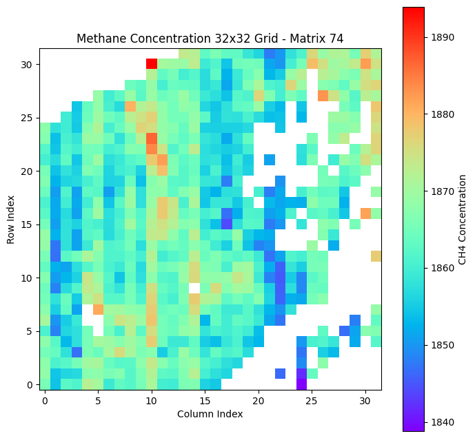

One of the images from the code.

If we want to plot the polygon data associated with these scenes, we need to extract the polygon data from the matrices we created. The following function organizes the data from a matrix.

def polygon_plot_params(matrix_):
    scene_lat_corners = []
    scene_lon_corners = []
    scene_ch4 = []
    for row in matrix_:
        for cell in row:
            # Check if the cell is not None and ch4 is not NaN
            if cell is not None and not np.isnan(cell['ch4']):  
                scene_lat_corners.append(cell['lat_corners'])
                scene_lon_corners.append(cell['lon_corners'])
                scene_ch4.append(cell['ch4'])


    # Bounding box values
    min_lon, max_lon, min_lat, max_lat = [np.min(scene_lon_corners),
                                          np.max(scene_lon_corners),
                                          np.min(scene_lat_corners),
                                          np.max(scene_lat_corners)]

    # Calculate current width and height
    width = max_lon - min_lon
    height = max_lat - min_lat

    # Desired aspect ratio
    aspect_ratio_width = 4
    aspect_ratio_height = 3

    # Determine which dimension needs to be increased
    # Calculate target width and height based on the dominant dimension
    if width / height < aspect_ratio_width / aspect_ratio_height:
        # Increase width to match the desired aspect ratio
        target_width = height * (aspect_ratio_width / aspect_ratio_height)
        target_height = height
    else:
        # Increase height to match the desired aspect ratio
        target_height = width * (aspect_ratio_height / aspect_ratio_width)
        target_width = width

    # Calculate the new boundaries
    center_lon = (min_lon + max_lon) / 2
    center_lat = (min_lat + max_lat) / 2

    new_min_lon = center_lon - target_width / 2
    new_max_lon = center_lon + target_width / 2
    new_min_lat = center_lat - target_height / 2
    new_max_lat = center_lat + target_height / 2

    # The new square bounding box values
    new_bounding_box = [new_min_lon, new_max_lon, new_min_lat, new_max_lat]
    # Define the increase amount
    increase_amount = 0.2

    # Adjusting the bounding box based on the direction and sign
    # We're adding to max values and subtracting from min values
    final_bounding_box = [
        new_bounding_box[0] - increase_amount,  # Decrease Min Lon
        new_bounding_box[1] + increase_amount,  # Increase Max Lon
        new_bounding_box[2] - increase_amount,  # Decrease Min Lat
        new_bounding_box[3] + increase_amount   # Increase Max Lat
    ]

    return scene_lat_corners, scene_lon_corners, scene_ch4, final_bounding_boxC

We then need a function that will prepare the plots of the polygons with a basemap. Here, I used one of the Blue Marble images, which can be found and downloaded from NASA’s website.

def plot_polygons_with_basemap(ax, scene_lat_corners, scene_lon_corners, scene_ch4, final_bounding_box):

    m = Basemap(llcrnrlon= final_bounding_box[0], llcrnrlat=final_bounding_box[2],
                urcrnrlat=final_bounding_box[3], urcrnrlon=final_bounding_box[1], ax=ax, projection='cyl')

    # Display the blue marble image
    m.warpimage(image='land_ocean_ice_8192.png')
    m.drawcoastlines(linewidth=0.2)
    m.drawcountries(linewidth=0.2)

    # Normalize the ch4 values for the colormap
    norm = mcolors.Normalize(vmin=min(scene_ch4), vmax=max(scene_ch4))
    cmap = colormaps['rainbow']

    # Plot the grid cells and color them based on ch4 values
    for lat_corners, lon_corners, ch4_value in zip(scene_lat_corners, scene_lon_corners, scene_ch4):
        color = cmap(norm(ch4_value))
        poly = Polygon(list(zip(lon_corners, lat_corners)), facecolor=color,
                       edgecolor='grey', linewidth=0.1, alpha=0.9)
        ax.add_patch(poly)

    # Set axis labels and ticks
    #ax.set_xlabel('Longitude')
    #ax.set_ylabel('Latitude')
    # Generate ticks and round them
    x_ticks = np.round(np.linspace(final_bounding_box[0], final_bounding_box[1], num=4), 2)
    y_ticks = np.round(np.linspace(final_bounding_box[2], final_bounding_box[3], num=4), 2)

    ax.set_xticks(x_ticks)
    ax.set_yticks(y_ticks)

And finally, to tie it all together: plotting everything.

#some less important stuff for visualization that isnt necessary
#################################
viridis_big = mpl.colormaps['rainbow']
newcmp = ListedColormap(viridis_big(np.linspace(0.0, 1.0, 256)))

font_size = 'small'
font_size_large = 'small'

fraction = 0.0457
#################################

for idx, matrix in enumerate(ch4_matrices):
    fig, axs = plt.subplots(1, 3, figsize=(15, 4), dpi=150)

    #first plot
    scene_lat_corners, scene_lon_corners, scene_ch4, final_bounding_box = polygon_plot_params(matrix)
    plot_polygons_with_basemap(axs[0], scene_lat_corners, scene_lon_corners, scene_ch4, final_bounding_box)
    axs[0].set_xlabel('Longitude', fontsize=font_size)
    axs[0].set_ylabel('Latitude', fontsize=font_size)
    axs[0].tick_params(axis='both', which='major', labelsize=font_size)

    #second plot
    cax1 = axs[1].imshow(matrix['ch4'], cmap=newcmp, interpolation='nearest')
    cbar1 = fig.colorbar(cax1, ax=axs[1], orientation='vertical', fraction=fraction, pad=0.04)
    cbar1.ax.set_title('[ppb]', fontsize=font_size, pad=6)
    cbar1.ax.tick_params(labelsize=font_size)
    axs[1].invert_yaxis()
    axs[1].set_xticks(np.arange(0, matrix.shape[1], 5))
    axs[1].set_yticks(np.arange(0, matrix.shape[0], 5))
    axs[1].tick_params(axis='both', which='major', labelsize=font_size)


    # Third plot with normalized parameters (e.g., different colormap)
    normalized_matrix = normalize_matrix(matrix['ch4'])
    cax2 = axs[2].imshow(normalized_matrix, cmap=newcmp, interpolation='nearest', vmin=0.0, vmax=np.max(normalized_matrix))
    cbar2 = fig.colorbar(cax2, ax=axs[2], orientation='vertical', fraction=fraction, pad=0.04)
    cbar2.ax.set_title('[-]', fontsize=font_size, pad=6)
    cbar2.ax.tick_params(labelsize=font_size)
    axs[2].invert_yaxis()
    axs[2].set_xticks(np.arange(0, matrix.shape[1], 5))
    axs[2].set_yticks(np.arange(0, matrix.shape[0], 5))
    axs[2].tick_params(axis='both', which='major', labelsize=font_size)

    plt.tight_layout()
    plt.show()