Non-Negative Matrix Factorization: A Complete Derivation from First Principles
Every formula proved. No gaps. No “it can be shown that…”
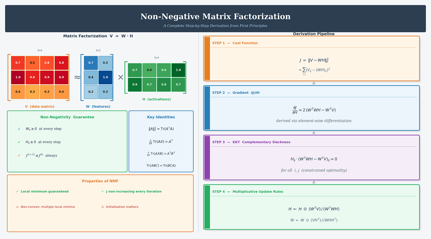
Non-Negative Matrix Factorization: A Complete Derivation from First Principles
Every formula proved. No gaps. No “it can be shown that…”
If you search for NMF derivations online, you will find one of two things: hand-wavy intuitions that skip the math, or dense papers that assume you already know everything. This article is neither. We go from the definition of a matrix norm all the way to the final update rules, proving every single intermediate step.
By the end you will know exactly why the update rule is what it is — not because someone told you, but because you derived it yourself.
-
What You Need to Know Before Starting
You need: basic matrix multiplication, partial derivatives, and the idea of minimisation. That’s it. Everything else — trace identities, Lagrange multipliers, the Kronecker delta — is derived here from scratch.
— -
Section 0 — Prerequisites and Notation
0.1 The Kronecker Delta
The Kronecker delta is a two-index function defined as:

Its most important use: it acts as a selector inside a sum.

When you sum over j, the delta forces j = k, killing all other terms. Only the j = k term survives.
- Why we care: When we differentiate element Xᵢⱼ with respect to element Xₘₙ, the answer is 1 only when both indices match:

This single identity is the engine of all matrix differentiation done here.
— -
0.2 The Four Trace Identities
The trace of a square matrix A is the sum of its diagonal elements: Tr(A) = Σᵢ Aᵢᵢ.
We will use four identities. Here they are — all proved below:

Proof of T1 (Tr(A) = Tr(Aᵀ)):
The (i,i) diagonal entry of Aᵀ is (Aᵀ)ᵢᵢ = Aᵢᵢ by definition of transpose. So both traces sum the same diagonal entries. ∎
Proof of T2 (linearity):
Tr(A+B) = Σᵢ(A+B)ᵢᵢ = Σᵢ(Aᵢᵢ + Bᵢᵢ) = Tr(A) + Tr(B). ∎
Proof of T3 (cyclic property):
Write Tr(AB) = Σᵢ Σₖ AᵢₖBₖᵢ. Write Tr(BA) = Σᵢ Σₖ BᵢₖAₖᵢ. Relabelling i↔k in the second sum shows they are identical. Applying this twice gives Tr(ABC) = Tr(BCA). ∎
- Proof of T4 (Frobenius = trace):

The (j,j) entry of AᵀA is the sum of squares of column j of A. Summing over all j gives the sum of squares of all entries — which is exactly ‖A‖²_F. ∎
— -
Section 1 — The Problem Setup
1.1 What is NMF?
Given a non-negative data matrix V of size m×n, find two non-negative matrices W (m×k) and H (k×n) such that:

where:

k is small — it is the number of hidden “features.” Think of V as a dataset of movie ratings. W describes what each latent feature looks like. H describes how strongly each feature activates for each user. Non-negativity means features only add — there is no negative cancellation, giving interpretable, parts-based representations.
1.2 The Cost Function
We measure how bad our approximation is using the squared Frobenius norm — simply the sum of squared element-wise differences:

J = 0 means perfect reconstruction. We want J as small as possible subject to W ≥ 0 and H ≥ 0:

This is a constrained optimisation problem. The constraint W, H ≥ 0 is what makes it hard, and is what prevents us from just running standard gradient descent.
— -
Section 2 — Expanding the Frobenius Norm
Before we can differentiate J, we need to expand ‖V − WH‖² into a form that is easy to differentiate. We convert it into trace form using Identity T4.
Step 1 — Apply T4
Set A = V − WH in T4 (‖A‖²_F = Tr(AᵀA)):

Step 2 — Expand the Transpose
Use (A − B)ᵀ = Aᵀ − Bᵀ and the rule (WH)ᵀ = HᵀWᵀ (reverse order on transpose of a product):

Step 3 — Multiply Out the Brackets
Expand exactly like (a − b)(a − b) = a² − ab − ba + b², but for matrices:

Apply T2 (linearity of trace) to split into four separate traces:

Step 4 — Combine the Middle Two Terms
Claim: Tr(HᵀWᵀV) = Tr(VᵀWH).
Proof: Use T1 — Tr(M) = Tr(Mᵀ). Set M = HᵀWᵀV. Then Mᵀ = (HᵀWᵀV)ᵀ = VᵀWH (reverse order, each transposed). So Tr(HᵀWᵀV) = Tr(VᵀWH). ∎
Therefore the two middle terms add up:

Step 5 — Simplify the Last Term
Use the cyclic property T3 to rewrite the last term in a cleaner order:

(Move Hᵀ from the front to the back of the trace cycle.)
Final Expanded Form
Putting it all together:

This is J written purely in terms of trace operations — now we can differentiate it.
— -
Section 3 — Gradient ∂J/∂H
We differentiate each of the three terms of J with respect to H, element by element. The key tool is: for each (m, n), compute ∂J/∂Hₘₙ, then assemble the matrix ∂J/∂H from all these scalars.
Term 1 — ∂/∂H ‖V‖² = 0.
‖V‖² contains no H. Every derivative is zero.
Term 2 — ∂/∂H [−2 Tr(VᵀWH)]
We first derive the general rule ∂/∂X Tr(AX) = Aᵀ from scratch:

Walk through line by line:- Line 1: Write Tr(AX) as an explicit double sum using the definition of matrix multiplication.
-
Line 2: Differentiate w.r.t. Xₘₙ. The only element of X that appears is Xₖᵢ, and its derivative w.r.t. Xₘₙ is the Kronecker delta δₖₘ · δᵢₙ.
-
Line 3: Apply the two deltas — they force k = m and i = n, killing every other term. Only Aₙₘ survives.
-
Line 4: Aₙₘ = (Aᵀ)ₘₙ, and since this holds for every (m, n), the matrix derivative is Aᵀ.
Applying with A = VᵀW and X = H:

Term 3 — ∂/∂H Tr(WᵀWHHᵀ)
Let B = WᵀW (constant w.r.t. H, and symmetric: Bᵀ = B). We derive the rule ∂/∂H Tr(BHHᵀ) = 2BH from scratch:

Walk — Line 1: Write Tr(BHHᵀ) as a triple sum over indices i, j, s.
-
Line 2: Differentiate the product Hⱼₛ · Hᵢₛ using the product rule. Each factor contributes one Kronecker delta pair.
-
Lines 3–4: Apply the deltas to each part separately. Part A (from the first delta pair) gives (BH)ₘₙ. Part B (from the second pair) also gives (BH)ₘₙ. Both use the fact that B is symmetric, so Bᵀ = B.
-
Line 5: Add Part A and Part B → result is 2(BH)ₘₙ for every (m, n), so the matrix derivative is 2BH.
Substituting B = WᵀW:

Assembling ∂J/∂H
Add all three terms:

— -
Section 4 — Gradient ∂J/∂W
Same approach, now differentiating with respect to W.
Term 2 — ∂/∂W [−2 Tr(VᵀWH)]
We need the rule ∂/∂X Tr(AXB) = AᵀBᵀ, derived the same way:

The logic is identical: write as a triple sum, apply ∂Xⱼₖ/∂Xₘₙ = δⱼₘ δₖₙ, the two deltas collapse the sum to a single term.
Applying with A = Vᵀ, X = W, B = H:

Term 3 — ∂/∂W Tr(WᵀWHHᵀ)
Let C = HHᵀ (symmetric). Same element-wise product-rule argument as before gives:

Assembling ∂J/∂W

— -
Section 5 — Why Plain Gradient Descent Fails
Standard gradient descent would update H as:
H ← H − α · 2(WᵀWH − WᵀV)
The problem: If Hₘₙ = 0.01 and the gradient at (m, n) is +10, then with α = 0.05:
H_mn ← 0.01 − 0.05 × 10 = −0.49 ← NEGATIVE. Constraint violated!
Plain gradient descent destroys non-negativity. We need to handle the constraint H ≥ 0 mathematically. The correct tool is the KKT conditions.
— -
Section 6 — KKT Conditions
6.1 Rewrite the Constraint
KKT handles inequality constraints in the form g(x) ≤ 0. Our constraint Hᵢⱼ ≥ 0 becomes:

6.2 The Lagrangian
Introduce a Lagrange multiplier λᵢⱼ ≥ 0 for each constraint. The Lagrangian is the objective plus each constraint multiplied by its multiplier:

6.3 The Four KKT Conditions
At any local minimum, all four conditions must hold simultaneously:

Unpacking each condition:
Condition 1 (Stationarity): The Lagrangian has zero gradient. This connects λᵢⱼ to the gradient of J.
Condition 2 (Primal Feasibility): The solution must satisfy H ≥ 0.
Condition 3 (Dual Feasibility): The multipliers λᵢⱼ ≥ 0. Substituting Condition 1 means the gradient of J cannot be negative at the optimum — otherwise we could still decrease J by moving further.
- Condition 4 (Complementary Slackness): This is the most powerful. Substituting λᵢⱼ from Condition 1:

This says: either Hᵢⱼ = 0 (we are on the boundary) or the gradient is zero (we are at an interior minimum). Both cannot be nonzero at once.
The two cases:
Case A: Hᵢⱼ > 0 → gradient must be 0 → (WᵀWH)ᵢⱼ = (WᵀV)ᵢⱼ. Standard unconstrained optimum.
Case B: Hᵢⱼ = 0 → gradient ≥ 0. J would increase if we pushed H below 0, but the constraint prevents it. We stay at the boundary.
— -
Section 7 — From KKT to the Multiplicative Update Rule
7.1 Rearrange the KKT Condition (Pure Algebra)
Start from complementary slackness and expand the bracket:

Line by line:
-
Line 1: Expand Hᵢⱼ · (WᵀWH − WᵀV)ᵢⱼ = 0 by distributing Hᵢⱼ.
-
Line 2: Move the negative term to the right side.
-
Line 3: Divide both sides by (WᵀWH)ᵢⱼ.
This is a fixed-point equation. The optimal H satisfies Hᵢⱼ = Hᵢⱼ · (WᵀV)ᵢⱼ / (WᵀWH)ᵢⱼ. No assumption was made — this is pure algebraic rearrangement of KKT.
7.2 Fixed-Point Iteration
A classical technique: if the solution satisfies x = f(x), then iterate x ← f(x) to find it. Apply this directly:


where ⊙ means element-wise multiplication and / means element-wise division.
These are the NMF multiplicative update rules. They were not pulled from thin air — they emerged directly from the KKT fixed-point equation.
7.3 Verify: Fixed Point Satisfies KKT
At convergence H = H · (WᵀV) / (WᵀWH):
-
If H**ᵢⱼ > 0: Divide both sides by Hᵢⱼ → ratio equals 1 → (WᵀWH)ᵢⱼ = (WᵀV)ᵢⱼ → gradient = 0. ✓ KKT Case A satisfied.
-
*If Hᵢⱼ = 0:** Left side = 0, right side = 0 · (ratio) = 0. ✓ KKT Case B satisfied trivially.
— -
Section 8 — Non-Negativity Is Preserved
Claim: If W ≥ 0, H ≥ 0, V ≥ 0 at step t, then H ≥ 0 at step t+1.
Proof by induction:
Base case (t = 0): Initialise W and H with small random positive values. ✓
Inductive step: Assume H⁽ᵗ⁾ ≥ 0. After the update:
-
Numerator (WᵀV)ᵢⱼ = Σₖ Wₖᵢ Vₖⱼ. Each term Wₖᵢ ≥ 0 (by hypothesis) and Vₖⱼ ≥ 0 (given data). Sum of non-negatives ≥ 0. ✓
-
Denominator (WᵀWH)ᵢⱼ = Σₖ (WᵀW)ᵢₖ Hₖⱼ⁽ᵗ⁾. Each factor ≥ 0. Sum ≥ 0. ✓
Therefore H⁽ᵗ⁺¹⁾ = H⁽ᵗ⁾ · [non-negative / non-negative] ≥ 0. ✓
An identical argument applies to W.
— -
Section 9 — Convergence: J Never Increases
9.1 The Auxiliary Function Method
Lee and Seung (1999) proved convergence using an auxiliary function G(H, H_old):
-
Property P1: G(H, H_old) ≥ J(H) for all H, H_old — G is an upper bound on J.
-
Property P2: G(H, H) = J(H) for all H — G is tight on the diagonal.
-
The key theorem: If we define each update as H⁽ᵗ⁺¹⁾ = argminₕ G(H, H⁽ᵗ⁾), then:

Reading the chain: 1. J(H⁽ᵗ⁺¹⁾) ≤ G(H⁽ᵗ⁺¹⁾, H⁽ᵗ⁾) by Property P1.
-
G(H⁽ᵗ⁺¹⁾, H⁽ᵗ⁾) ≤ G(H⁽ᵗ⁾, H⁽ᵗ⁾) because H⁽ᵗ⁺¹⁾ minimises G.
-
G(H⁽ᵗ⁾, H⁽ᵗ⁾) = J(H⁽ᵗ⁾) by Property P2.
Therefore J is non-increasing at every step. Since J ≥ 0, it must converge.
9.2 The Update Rule Minimises the Auxiliary Function
The auxiliary function is constructed by replacing the quadratic curvature in a Taylor expansion with a looser (but elementwise-separable) upper bound. For each (i, j) the relevant piece of G is:
g(H_ij) = constant

+ H_ij · [gradient of J at H^(t)]

+ [(WᵀWH^(t))_ij / H^(t)_ij] · (H_ij − H^(t)_ij)²
Setting dg/dHᵢⱼ = 0 and solving:

The minimiser of G is exactly the multiplicative update rule. This closes the loop: not only does our update converge, it does so by minimising a tight upper bound on J at every step.
— -
Section 10 — The Complete Algorithm
INPUT: V (m × n, non-negative)

k (number of latent features, k ≪ min(m,n))

STEP 1: Initialise W (m×k) and H (k×n) with small random positive values

STEP 2: Repeat until convergence:

UPDATE H: H ← H ⊙ (WᵀV) / (WᵀWH)

UPDATE W: W ← W ⊙ (VHᵀ) / (WHHᵀ)

COMPUTE: J = ‖V − WH‖²_F

STOP if J has decreased by less than a tolerance ε

OUTPUT: W, H such that V ≈ WH, all entries ≥ 0
Guaranteed properties:
-
✅ Non-negativity of W and H preserved at every step.
-
✅ J is monotonically non-increasing.
-
✅ Fixed points of the update satisfy the KKT optimality conditions.
-
⚠️ NMF is not jointly convex in (W, H) — only local minima are guaranteed.
-
⚠️ Different random initialisations may give different solutions.
-
⚠️ Add a small ε to denominators to avoid division by zero.
— -
The Complete Logical Chain
GIVEN

Minimise J = ‖V − WH‖² subject to W, H ≥ 0

STEP 1 — Apply ‖A‖² = Tr(AᵀA)

J = ‖V‖² − 2 Tr(VᵀWH) + Tr(WᵀWHHᵀ)

STEP 2 — Differentiate term by term (element-wise + Kronecker delta)

∂J/∂H = 2(WᵀWH − WᵀV)

∂J/∂W = 2(WHHᵀ − VHᵀ)

STEP 3 — Observe plain GD violates H, W ≥ 0 → use KKT

STEP 4 — Write Lagrangian, apply all 4 KKT conditions

Complementary slackness: H_ij · (WᵀWH − WᵀV)_ij = 0 ∀ i,j

STEP 5 — Rearrange KKT algebraically into a fixed-point equation

H_ij = H_ij · (WᵀV)_ij / (WᵀWH)_ij

STEP 6 — Apply fixed-point iteration x ← f(x)

H ← H ⊙ (WᵀV)/(WᵀWH)

W ← W ⊙ (VHᵀ)/(WHHᵀ)

STEP 7 — Verify

Non-negativity preserved ✅

J decreases every step ✅

Converges to KKT ✅
— -
Summary
The multiplicative update rules are not a trick. They are the direct algebraic consequence of three things:
-
The gradient of the squared Frobenius cost.
-
The KKT complementary slackness condition for non-negativity.
-
Rearranging that condition into a fixed-point iteration.
Every symbol in the final formula traces back to a first-principles derivation. That is NMF — completely understood.
— -
메타데이터
- post_id
- 33f15716cd7a
- slug
- non-negative-matrix-factorization-a-complete-derivation-from-first-principles-33f15716cd7a
- url
- https://medium.com/@abhishekh_15857/non-negative-matrix-factorization-a-complete-derivation-from-first-principles-33f15716cd7a
- canonical_url
- https://medium.com/@abhishekh_15857/non-negative-matrix-factorization-a-complete-derivation-from-first-principles-33f15716cd7a
- author_url
- https://medium.com/@abhishekh_15857
- status
- ok
- fetched_at
- 2026-06-12 18:14:10




