Master Kubernetes Tracing: Grafana Tempo + Alloy Made Simple

Learn to Instrument, Visualize, and Analyze Distributed Traces with Grafana Tempo, Alloy, and Grafana — Build a Complete Tracing Pipeline from Scratch

Introduction: The Problem This Solves — Scenario: The 45-Minute Debugging Nightmare

You have just deployed a microservices application on your Kubernetes cluster. Everything seems fine until a user reports: “Checkout failed — again.”

You start debugging:

• Check the frontend pod logs — nothing unusual.
• Check the payment service logs — no errors.
• Check the inventory service — looks healthy.
• Check the notification service — wait, there is a timeout here. But why is notification even in the checkout flow?

45 minutes later, you discover the issue: a third-party email API called by the notification service is timing out, blocking the entire checkout process. You had all the logs, but you lacked context. You could not see how services connect, what depends on what, or where the real bottleneck was.

This is the problem distributed tracing solves — and Grafana Tempo is here to make it simple.

1. What Is Tracing? What Is Distributed Tracing?

Tracing (Simple Explanation)

Tracing is the process of tracking a request as it moves through your system.

When a user clicks “Checkout”, that single request does not stay in one place — it travels across multiple services like frontend, backend, payment, inventory, and database. Tracing helps you follow that entire journey end-to-end.

What Is a Trace?

A trace represents the complete lifecycle of a single request.

• It starts when the request enters your system
• It ends when the response is returned
• It includes every service and operation involved along the way

Think of a trace as the full story of a request.

What Is a Span?

A span is a single unit of work within a trace.

Examples of spans:

• An API call
• A database query
• A function execution
• A call to another service

If a trace is the full story, a span is one step in that story.

Parent and Child Spans (Hierarchy)

Spans are not isolated — they form a hierarchy.

• A parent span represents a higher-level operation
• A child span represents a smaller task inside it

For example:

• process-payment (parent span)
• encrypt-data (child span)
• call-payment-gateway (child span)
• wait-for-response (child span)

This creates a tree structure, where:

• One trace consists of many spans
• One span can contain multiple child spans

Trace (Checkout Request)
└── frontend (root span)
    ├── backend API
    │   ├── payment service
    │   └── inventory service
    └── notification service

What Is Distributed Tracing?

Distributed tracing extends this concept across multiple services.

Instead of tracking work inside a single service, it tracks:

• How a request moves across services
• Which service calls which
• How long each step takes

This works through context propagation, where a unique trace ID is passed between services, usually via HTTP headers.

Why Logs Alone Fail

Logs tell you what happened inside a single service.

But in distributed systems:

• A single request touches multiple services
• Logs are scattered across those services
• There is no built-in connection between them

This makes it difficult to answer:

• Which service caused the delay?
• What happened before the failure?
• Where did the request actually break?

Why Tracing Solves This

Tracing connects everything into a single view:

• Shows the full request flow
• Reveals service dependencies
• Highlights latency at each step
• Pinpoints the exact bottleneck

Instead of guessing, you can see the entire system behavior for a request in one place.

2. What Is Tempo? Why Use It?

Tempo is an open-source, scalable distributed tracing backend built by Grafana Labs. It is designed for cost-effective, large-scale trace storage.

Key benefits of Tempo:

• Cost-effective storage: Stores traces in object storage (S3, GCS, MinIO) instead of hot memory or expensive databases, dramatically reducing operational costs.
• No indexing: Does not index trace contents — only stores them. This eliminates the storage and compute overhead associated with indexing, making it possible to store massive volumes of traces.
• Native Grafana integration: Provides a seamless experience if you already use Grafana for metrics and logs, with no additional UI to learn or maintain.
• OpenTelemetry native: Accepts OTLP (OpenTelemetry Protocol) out of the box with no additional configuration or protocol translation.
• Unlimited scale: Object storage can scale indefinitely at low cost, meaning you never outgrow your tracing backend.

3. Tempo Architecture

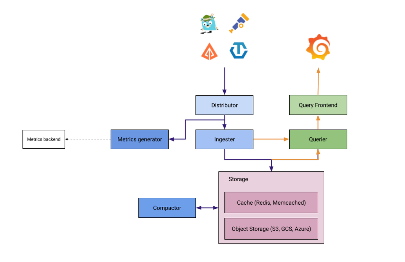
Tempo consists of several components that work together to ingest, store, and retrieve traces.

Component breakdown:

Distributor: Accepts spans from collectors via OTLP. It hashes each span by its traceID for consistent routing to ingesters. The distributor is stateless and can be scaled horizontally.

Ingester: Receives spans from distributors and batches them into blocks held in memory. When a block reaches a configured size or time threshold, it is flushed to object storage. Ingesters are stateful during the flushing process.

Querier: Fetches traces from both ingesters (for hot, recent data still in memory) and object storage (for cold, historical data). It merges results and returns complete traces to Grafana.

Compactor: Runs periodically to deduplicate, compress, and optimize blocks in object storage. It reduces storage costs and improves query performance by merging smaller blocks into larger, more efficient ones.

Query Frontend (optional): Handles query splitting, caching, and parallelization. It improves query performance for large-scale deployments by distributing work across multiple queriers.

Flow of a trace through the architecture:

• Instrumented application generates spans and sends them to Alloy.
• Alloy forwards spans via OTLP to the Distributor.
• Distributor hashes the traceID and forwards to the appropriate Ingester.
• Ingester writes spans to a block in memory.
• When the block is complete, Ingester flushes it to object storage.
• Compactor periodically optimizes blocks in storage.
• Developer queries in Grafana → Query Frontend → Querier.
• Querier fetches from Ingesters (hot data) and object storage (cold data).
• Complete trace is returned to Grafana for visualization.

Application → Alloy (Collector) → Distributor → Ingester → Object Storage
                                    ↓
                              Querier ← Compactor
                                    ↓
                              Grafana (UI)

4. How Tempo Works: Following a Single Request

• A user request hits your application’s entry point.
• Your instrumented application generates spans, all sharing a common traceID. Each span represents a discrete operation like an HTTP call, database query, or internal function.
• Alloy (or any OpenTelemetry collector) receives these spans from your application, either by receiving OTLP directly or by scraping OpenTelemetry endpoints.
• Alloy sends spans via OTLP (gRPC or HTTP) to Tempo’s Distributor.
• The Distributor hashes the traceID and forwards spans to the appropriate Ingester. This ensures all spans for the same trace go to the same ingester, keeping the trace together.
• The Ingester batches spans into blocks held in memory. Batching improves write efficiency and reduces object storage operations.
• When a block is complete (by size or time), it is flushed to object storage such as S3, GCS, MinIO, or local disk.
• The Compactor runs periodically to optimize blocks, removing duplicate data and merging smaller blocks into larger ones.
• A developer queries for a trace in Grafana. Grafana sends the request to the Querier (or Query Frontend).
• The Querier fetches the trace from ingesters for recent data and from object storage for historical data, then merges the results.
• The complete trace visualization appears in Grafana’s waterfall view, showing every span across every service.

5. Grafana Alloy: The Collector That Makes It Work

What is Alloy?

Alloy is Grafana’s vendor-agnostic telemetry collector. It is the successor to Grafana Agent and is designed for OpenTelemetry-native observability.

Why Alloy?

• Single agent for collecting traces, logs, metrics, and profiles from a single deployment, reducing agent sprawl.
• OpenTelemetry-native configuration that follows OpenTelemetry Collector standards, making it familiar to anyone who has used OTel.
• Kubernetes-native with automatic pod and service discovery using the Kubernetes API, eliminating manual configuration.
• Pipeline flexibility supporting filtering, batching, transforming, and routing telemetry data before it leaves the agent.

What Alloy does in this stack:

• Discovers pods and services in your Kubernetes cluster automatically using label selectors and annotations.
• Collects OpenTelemetry spans from instrumented applications, either by receiving OTLP directly or by scraping OpenTelemetry endpoints.
• Forwards spans to Tempo via OTLP, with configurable batching, retries, and compression.
• Optionally forwards logs to Loki and metrics to Prometheus alongside traces, creating a complete observability pipeline from a single agent.

6. Does Tempo Have Its Own UI?

No — and that is by design.

Tempo has no native user interface. Instead, it relies entirely on Grafana as its frontend. This design decision provides several benefits:

• Unified observability: Logs, metrics, and traces are all visualized in one place — Grafana. You do not switch between different UIs to understand a single request.
• Seamless correlation: Click a traceID in Loki logs to open the corresponding trace in Tempo. This workflow is built into Grafana and requires no custom scripting.
• Reduced maintenance: One UI to maintain instead of separate interfaces for logs, metrics, and traces. This reduces operational overhead.
• Consistent user experience: The same query interface, visualization patterns, and dashboarding capabilities apply across all telemetry types.

7. Tempo vs. Jaeger: When to Use What

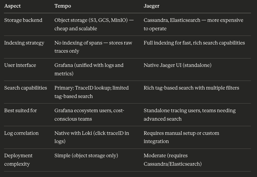
When to choose Tempo:

• You are already using Grafana, Loki, and Prometheus in your stack
• You want cost-effective long-term trace storage at scale
• Log-to-trace correlation is a high priority
• You primarily search by trace ID or service name rather than arbitrary tags

When to choose Jaeger:

• You need rich tag-based search with complex filtering
• You want a standalone tracing UI without dependency on Grafana
• You are already invested in Cassandra or Elasticsearch
• Your team is familiar with Jaeger’s native workflow

8. Project Structure and File Explanations

Before deploying, understand the complete project structure and what each file does.

Project Directory Structure

tempo-alloy-demo/
├── kind-config.yaml
├── trace-generator.yaml
├── helm/
│   ├── alloy-values.yaml
│   ├── prometheus-stack-values.yaml
│   └── tempo-values.yaml

File-by-File Explanation

kind-config.yaml — KIND Cluster Configuration

This file defines your local Kubernetes cluster. It creates one control-plane node and two worker nodes. KIND runs Kubernetes inside Docker containers, giving you a production-like cluster on your laptop.

kind: Cluster
apiVersion: kind.x-k8s.io/v1alpha4
name: tempo-demo
nodes:
  - role: control-plane
  - role: worker
  - role: worker

trace-generator.yaml — Trace Generator Deployment

This file deploys a k6-based trace generator that continuously sends synthetic traces to Alloy. It uses the xk6-client-tracing image which simulates microservice traffic. The key environment variable ENDPOINT points to alloy:4317, the OTLP gRPC endpoint where Alloy receives traces.

apiVersion: apps/v1
kind: Deployment
metadata:
  name: k6-trace-generator
  namespace: monitoring
spec:
  replicas: 1
  selector:
    matchLabels:
      app: k6-trace-generator
  template:
    metadata:
      labels:
        app: k6-trace-generator
    spec:
      containers:
      - name: k6-tracing
        image: ghcr.io/grafana/xk6-client-tracing:v0.0.7
        env:
        - name: ENDPOINT
          value: "alloy:4317"
        resources:
          limits:
            cpu: 200m
            memory: 256Mi
          requests:
            cpu: 100m
            memory: 128Mi
      restartPolicy: Always
---
apiVersion: v1
kind: Service
metadata:
  name: k6-trace-generator
  namespace: monitoring
spec:
  selector:
    app: k6-trace-generator
  ports:
  - port: 8080
    targetPort: 8080
    name: http
  type: ClusterIP

helm/alloy-values.yaml — Alloy Configuration

This file configures Grafana Alloy. It defines an OTLP receiver on ports 4317 (gRPC) and 4318 (HTTP) for incoming spans, then exports those spans to Tempo. The extraPorts section exposes these ports as Kubernetes services so other pods can send traces.

alloy:
  configMap:
    content: |
      otelcol.receiver.otlp "otlp_receiver" {
        grpc {
          endpoint = "0.0.0.0:4317"
        }
        http {
          endpoint = "0.0.0.0:4318"
        }
        output {
          traces = [otelcol.exporter.otlp.tempo.input]
        }
      }
      otelcol.exporter.otlp "tempo" {
        client {
          endpoint = "tempo:4317"
          tls {
            insecure = true
          }
        }
      }
  extraPorts:
    - name: otlp-grpc
      port: 4317
      targetPort: 4317
      protocol: TCP
    - name: otlp-http
      port: 4318
      targetPort: 4318
      protocol: TCP

helm/prometheus-stack-values.yaml — Prometheus + Grafana Configuration

Key configurations in this file:

• enableRemoteWriteReceiver: true — Allows Tempo's metrics generator to write metrics to Prometheus.
• exemplar-storage and native-histograms — Enable features that link metrics to traces via exemplars.
• Anonymous access in Grafana — Disables login for demo simplicity.
• TraceQL editor — Enables the advanced TraceQL query editor in Grafana.
• Tempo datasource — Automatically configures Grafana to connect to Tempo at [http://tempo:3200.](http://tempo:3200.)

prometheus:
  prometheusSpec:
    # Enable remote write receiver for Tempo metrics (default: false)
    enableRemoteWriteReceiver: true
    # Enable exemplar storage for metrics-traces linking (default: [])
    enableFeatures:
      - exemplar-storage
      - native-histograms

grafana:
  # Enable anonymous access for demo (default: requires login)
  grafana.ini:
    auth.anonymous:
      enabled: true
      org_role: Admin
    auth:
      disable_login_form: true
    feature_toggles:
      enable: traceqlEditor

  # Add trace exploration plugin (default: no plugins)
  plugins:
    - grafana-exploretraces-app

  # Connect Grafana to Tempo (default: only Prometheus datasource)
  datasources:
    datasources.yaml:
      apiVersion: 1
      datasources:
        - name: Tempo
          type: tempo
          access: proxy
          url: http://tempo:3200
          uid: tempo
          jsonData:
            httpMethod: GET
            serviceMap:
              datasourceUid: prometheus
            tracesToMetrics:
              datasourceUid: prometheus

# Disable components for simpler demo setup
alertmanager:
  enabled: false  # Default: true

nodeExporter:
  enabled: false  # Default: true

prometheus-node-exporter:
  enabled: false  # Default: true

helm/tempo-values.yaml — Tempo Configuration

Key configurations:

• metricsGenerator.enabled: true — Enables Tempo's metrics generator, which creates metrics from trace data automatically.
• remoteWriteUrl — Points to Prometheus so the metrics generator can write derived metrics.
• processors: [service-graphs, span-metrics, local-blocks] — Enables service graph generation, span metrics calculation, and local block storage.
• persistence.enabled: true — Enables persistent storage for traces.

tempo:
  # Specific commit for reproducibility
  tag: main-814c1c6

  # Metrics generator - The key feature for traces → metrics integration
  metricsGenerator:
    enabled: true
    remoteWriteUrl: "http://monitoring-kube-prometheus-prometheus:9090/api/v1/write"

  # Enable service graphs and span metrics
  overrides:
    defaults:
      metrics_generator:
        processors: [service-graphs, span-metrics, local-blocks]

# Enable persistence for realistic setup
persistence:
  enabled: true

9. Hands-On Demo: Deploying Tempo + Alloy on kind

Prerequisites

• kind (Kubernetes in Docker)
• kubectl
• helm

Step-by-Step Deployment

Step 1: Create kind cluster

kind create cluster --name tempo-demo --config kind-config.yaml
kubectl cluster-info --context kind-tempo-demo

Step 2: Create namespace

kubectl create namespace monitoring

Step 3: Add Helm repositories

helm repo add grafana-community https://grafana-community.github.io/helm-charts
helm repo add prometheus-community https://prometheus-community.github.io/helm-charts
helm repo update

Step 4: Deploy Prometheus + Grafana

helm install monitoring prometheus-community/kube-prometheus-stack \
  --version 82.18.0 \
  --namespace monitoring \
  --values helm/prometheus-stack-values.yaml \
  --wait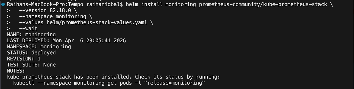

Step 5: Deploy Tempo

helm install tempo grafana-community/tempo \
  --version 2.0.0 \
  --namespace monitoring \
  --values helm/tempo-values.yaml \
  --wait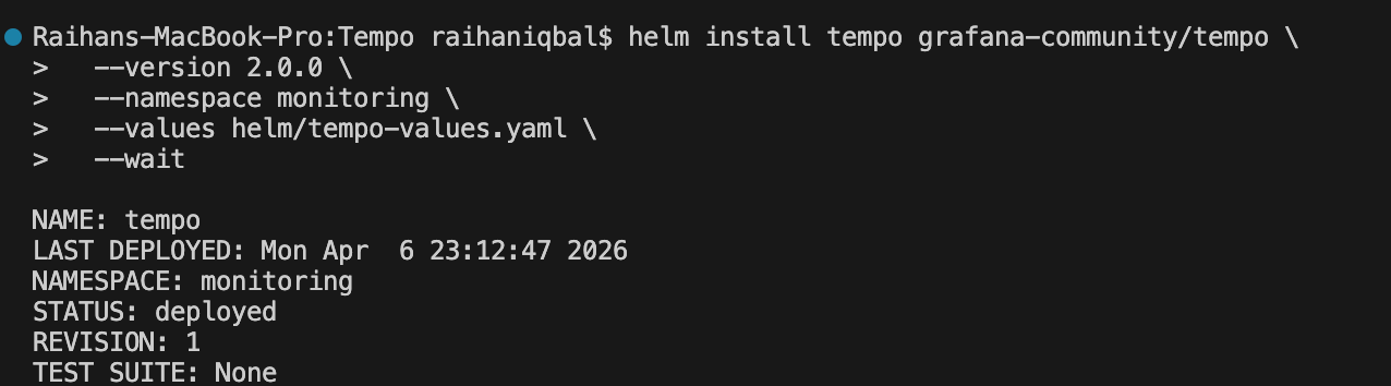

Step 6: Deploy Alloy

helm install alloy grafana/alloy \
  --version 1.7.0 \
  --namespace monitoring \
  --values helm/alloy-values.yaml \
  --wait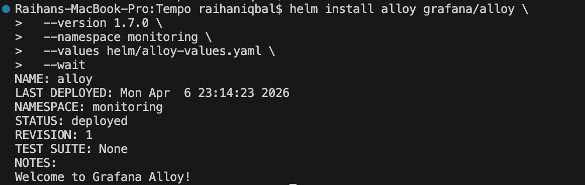

Step 7: Deploy trace generator

kubectl apply -f trace-generator.yaml

Step 8: Verify all pods are running

kubectl get pods -n monitoring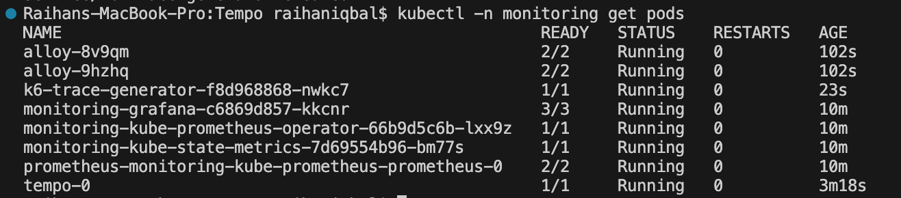

Verify that all pods show Running or Completed status. You should see pods for Prometheus, Grafana, Tempo components (distributor, ingester, querier, compactor), Alloy, and the k6 trace generator.

Step 9: Access Grafana UI

kubectl get svc -n monitoring
kubectl port-forward svc/monitoring-grafana 3000:80 -n monitoring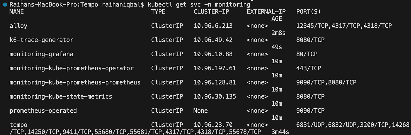

Access Grafana at: http://127.0.0.1:3000

Step 10: Verify Tempo data source in Grafana

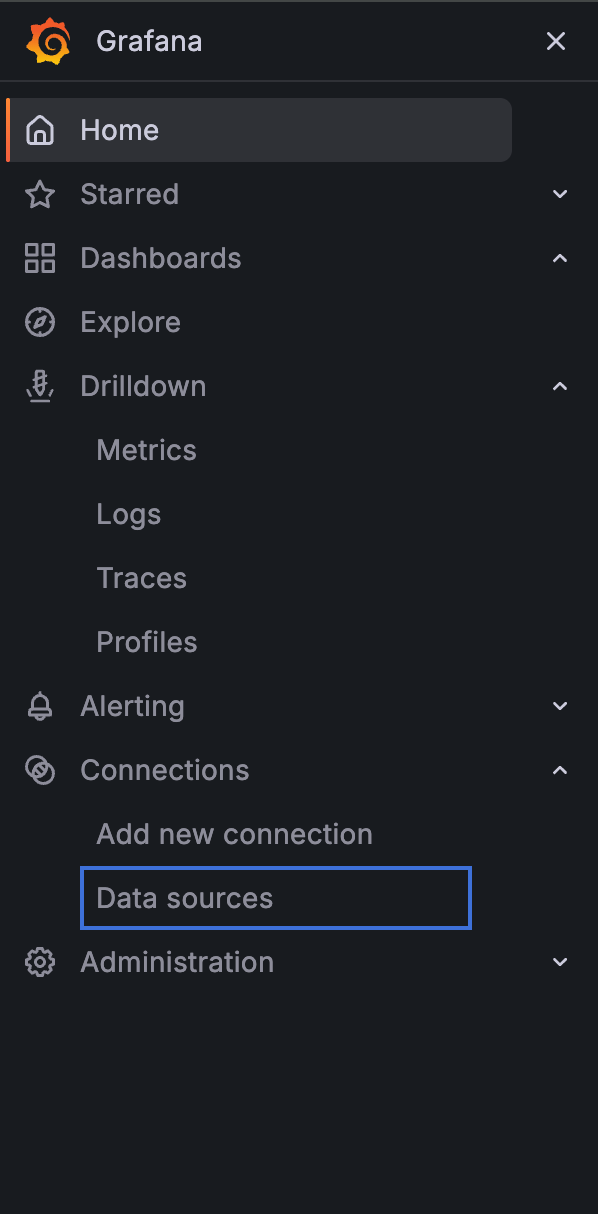
Log into Grafana. Anonymous access is enabled so no login is required. Click the menu icon on the left side, navigate to Configuration → Data Sources, and verify that Tempo appears as a configured data source.

Step 11: Explore traces in Grafana

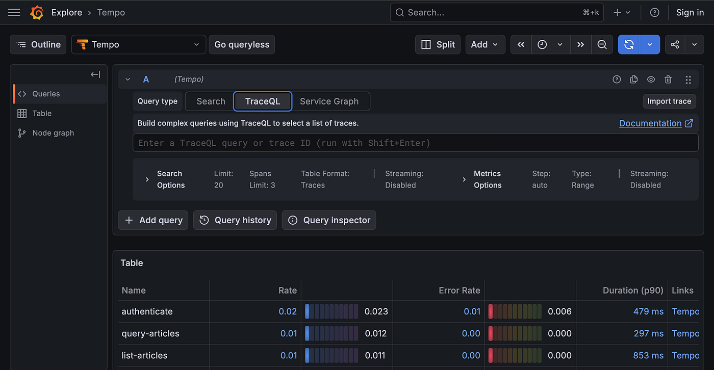
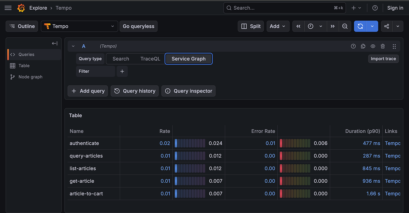
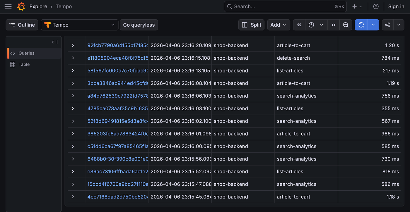
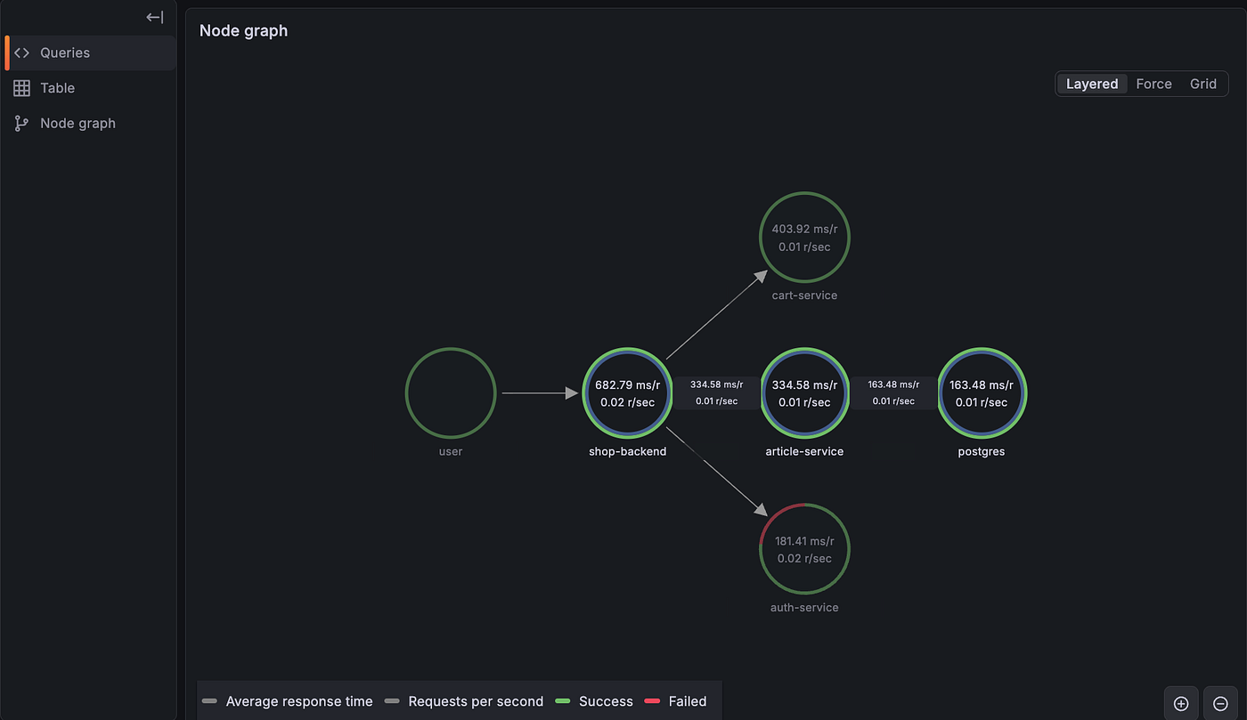
Click the Explore icon (compass) in the left sidebar and select Tempo as the data source. You will see three tabs: Search, TraceQL, and Service Graph. In the Search tab, select a service such as shop-backend or cart-service and click Run query. Click on any trace to open the waterfall visualization showing all spans and their parent-child relationships. Navigate to the Service Graph tab to see an interactive graph of service dependencies.

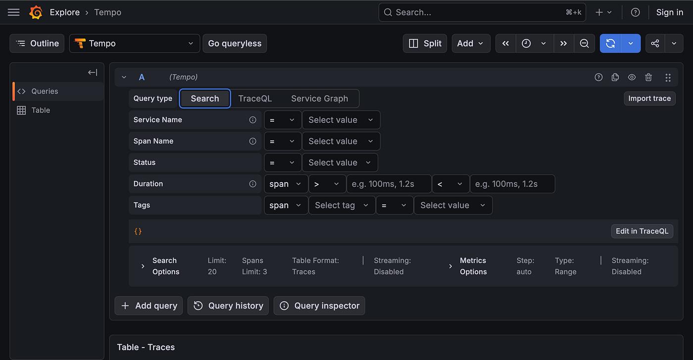
Step 12: View metrics from traces

In Grafana Explore, switch the data source to Prometheus and query for metrics generated by Tempo’s metrics generator such as traces_service_graph_request_total or traces_spanmetrics_latency_bucket. These metrics are created automatically from your trace data, giving you aggregated insights without any additional instrumentation on your part.

10. Understanding the Trace Output

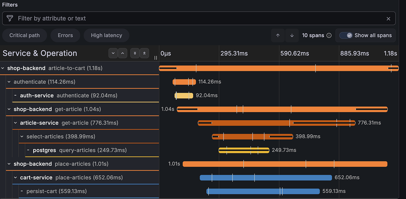
When you deploy this stack and open Grafana’s Explore view with Tempo selected, you will see a two-panel waterfall visualization like the screenshots below. The left panel shows the span hierarchy with service names and durations. The right panel shows the same spans as horizontal bars on a timeline, so you can see exactly when each span started and how long it ran relative to the total trace duration.

Span hierarchy from this trace:

Understanding Trace Visualization: A Practical Example

Let’s break down how to read a real trace visualization and extract meaningful insights to solve performance bottlenecks.

1. The Trace Interface

At the top of most modern observability platforms (like Jaeger, Honeycomb, or Datadog), you’ll find a Filters Bar. This allows you to slice through noise by selecting:

• Critical Path: Highlights the sequence of spans that determine the total duration.
• Errors: Filters for failed spans (usually marked in red).
• High Latency: Isolates spans exceeding a specific percentile (e.g., p95).
• Span Count: Shows the complexity of the request (e.g., 10 spans).

Below the filters is the Timeline, marked with millisecond increments (e.g., 295ms, 590ms, 1.18s). On the left, you see the Service Hierarchy; on the right, the Gantt Chart visualization of span durations.

2. Deconstructing the Hierarchy

The Root Span is your starting point. In our example, shop-backend article-to-cart takes 1.18 seconds. This is the total "wall-clock time" the user waits. Every other span is a child operation nested within this window.

The Authenticate Operation (Fast)

The shop-backend authenticate span took 114.26ms.

• It called auth-service authenticate, which took 92.04ms.
• The Delta: The ~22ms gap represents local processing (serialization/deserialization) within the shop-backend before and after the network call.

The Get-Article Operation (Slowest)

At 1.04 seconds, this is your primary bottleneck.

• It called article-service get-article (776.31ms).
• Inside that service, select-articles took 398.99ms, which eventually hit the database.
• The Leaf Span: The postgres query-articles took 249.73ms. This is the "end of the line"—the actual work being done at the data layer.

The Place-Articles Operation (High Overhead)

The shop-backend place-articles span took 1.01 seconds.

• It called cart-service place-articles (652.06ms).
• The Red Flag: There is a 358ms discrepancy between the parent and child. This suggests “unaccounted-for time” — likely heavy data transformation, uninstrumented internal functions, or perhaps a thread being blocked.

3. What the Trace Reveals

Logs tell you what happened; traces tell you where the time went. Two key insights emerge:

1. Database Inefficiency: The get-article path is bogged down by a 250ms Postgres query. This is a classic "low-hanging fruit" fix—likely solved by an index or query optimization.
2. Service Overhead: The 358ms of unexplained latency in shop-backend during the place-articles phase is a "silent killer." Without tracing, you’d likely blame the cart-service, but the trace proves the bottleneck is actually in the calling service’s logic.

4. Using Color Coding as a Map

Modern tracing uses color to denote Service Ownership:

• Orange: shop-backend
• Blue: Downstream services (cart-service, article-service)
• Yellow: Third-party/Infrastructure (postgres, auth-service)

Pro-Tip: If you see a long bar of one color followed by a tiny bar of another, the parent service is doing heavy computation. If you see a tiny bar followed by a massive bar of a different color, the parent is “I/O bound” (waiting on a dependency).

5. The Debugging Workflow

A trace transforms debugging from a “guessing game” into a surgical strike:

1. Observe: Identify the root latency (1.18s).
2. Isolate: Notice authenticate is healthy, but get-article is dragging.
3. Drill-Down: Follow the chain to the leaf span (postgres query-articles).
4. Pinpoint: Identify the specific query taking 249ms.
5. Remediate: Add the index or optimize the code.

The Bottom Line

Tracing provides the context of connectivity. It connects the dots between isolated logs, showing you the complete story of a request across every service and database. In a microservices world, it’s the difference between five minutes of debugging and five hours of finger-pointing.

11. Log-to-Trace Correlation: The Magic

Log-to-trace correlation is the ability to jump directly from a log entry to the full distributed trace that generated it. When a log line contains a traceID, you can click that ID and see every span across every service involved in that request.

How it works:

Your application logs include the current traceID in each log line, injected by the tracing SDK into the logging context. Alloy collects these logs and forwards them to Loki. In Grafana Explore with Loki as the data source, log lines show the traceID as a clickable link. Clicking it automatically switches to the Tempo data source and queries for that exact trace.

Example workflow:

Step 1 — Find a suspicious log in Loki:

2025-01-15 14:32:18 ERROR payment-service: timeout calling inventory API, traceID=abc123def456

Step 2 — Click the traceID. Grafana automatically switches to Tempo and queries for traceID=abc123def456.

Step 3 — View the complete trace. You see Frontend span taking 2.1 seconds total, Payment span taking 2.0 seconds calling inventory, Inventory span taking 1.9 seconds waiting on a database, and Database span taking 1.8 seconds on a slow query.

Step 4 — Identify root cause. The database query was unoptimized. You found the problem in seconds, not minutes.

Without correlation: find a log with an error, guess which trace matches, manually search for the trace ID, no cross-service context at all. With correlation: find the log, click the traceID, automatically retrieve the trace, see the full distributed context immediately.

12. Conclusion

You started with a 45-minute debugging nightmare — a checkout failure hiding in an unrelated notification service with no visibility across your microservices.

Now, with Grafana Tempo and Alloy, you have a complete distributed tracing pipeline running in Kubernetes, cost-effective storage using object storage instead of expensive databases, seamless log-to-trace correlation in Grafana, service graphs that reveal hidden dependencies at a glance, and the ability to answer not just “what happened?” but “why did it happen across 10 services?”

Key takeaways:

• Tempo brings production-ready tracing without breaking your budget using object storage.
• Alloy simplifies collection with a single agent for traces, logs, and metrics.
• Grafana ties it all together — logs, metrics, and traces in one unified interface.
• Service graphs reveal hidden dependencies and bottlenecks instantly.
• Log-to-trace correlation turns logs into clickable entry points for full trace investigation.

Observability is not about collecting as much data as possible. It is about asking the right questions and getting answers fast. With Tempo, you can stop guessing and start tracing.