Real-Time Stock Market Anomaly Detection Using Machine Learning: An End-to-End Data Engineering Project

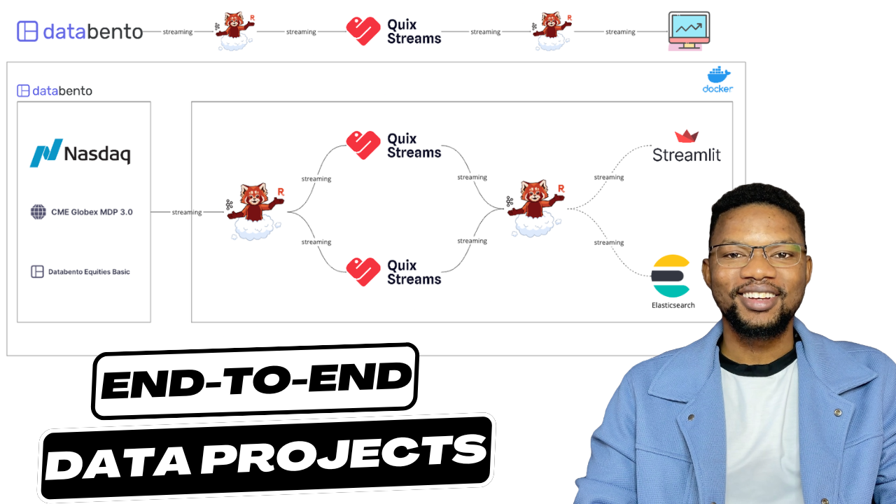
Identifying anomalies in real-time can make or break trading strategies especially in a fast paced industry like the stock market. From unusual price swings to abnormal trading volumes, the ability to detect these anomalies early can help mitigate risks and seize opportunities. In this article, we’ll explore how to build a real-time stock market anomaly detection system using machine learning models. This end-to-end project will walk you through everything from setting up the data pipeline to building, training and retraining an Isolation Forest model for anomaly detection.

In short, in this article we’ll cover:

• System Architecture Overview
• Ingesting Stock Market Data via FTP
• Setting Up a Real-Time Data Pipeline with Quix Streams
• Building the Anomaly Detection Model with Isolation Forest
• Testing the System and Analysing Results

For folks interested in a video walkthrough, you can catchup here

[embed]

System Architecture Overview

Our architecture centers around a streaming-first approach, ensuring real-time data ingestion and anomaly detection. Here’s a high-level breakdown of the system components:

• Data Ingestion: Stock market data is downloaded from Databento using FileZilla and then streamed into the pipeline using a Python producer.
• Data Pipeline: We’ll use the open source Python library **Quix Streams to handle the real-time processing and streaming of stock data into a Kafka** topic.
• Anomaly Detection: An Isolation Forest machine learning model will be used to identify irregularities in stock data.
• Monitoring and Output: Detected anomalies will be pushed to an alert system or visualised for decision-making.

Ingesting Stock Market Data with Databento and FileZilla

The first step in this project is to download stock market data from Databento using FileZilla. Databento is a popular data provider for stock market and financial datasets, offering comprehensive time series data for multiple asset classes.

After downloading the CSV files using FileZilla, we’ll use a Python producer to stream the data into our real-time pipeline. Here’s how to set up the data ingestion:

Downloading the Stock Data via FileZilla

1. Open FileZilla and connect to Databento’s FTP server using your login credentials.
2. Navigate to the folder containing the stock market data you want to download.
3. Download the CSV files to a local directory on your system. These files will contain columns such as timestamp, open, high, low, close, and volume, which will be used for our analysis.

Setting up Data Producer

Once the data is downloaded, we need to stream it into our pipeline. We’ll use Redpanda(Kafka) as our message broker and QuixStreams to handle the real-time processing. Together, these tools allow us to ingest, process, and analyze stock data with low latency and high throughput. Here’s how to set up a Python producer that streams the stock data into a Kafka topic.

Why Redpanda (Kafka)?

Redpanda is a great choice for modern data streaming due to its performance optimizations over traditional Kafka brokers. It delivers Kafka’s API compatibility but with reduced operational overhead, which means you can handle large-scale data without the need for Zookeeper or complex configurations.

Why Quix Streams?

Quix Streams makes real-time data ingestion, processing, and streaming more accessible by offering a user-friendly API that simplifies complex tasks. Its tight integration with Redpanda/Kafka allows for seamless streaming, and it provides built-in support for timeseries data and event-based architectures — perfect for stock market data.

Setting up a Python Producer for Stock Data Streaming

Before we switch gears and get into the code, you need to have QuixCLI (you can get it installed here) installed once installed. You can get the base project setup with:

quix init

quix project initialization

Once the initialisation is done, you can create the stock data producer using:

quix app create

As the producer is the source, we will be choosing the starter source, hence, we will be asked for the application name (which will be **producer) and output topic, in our case, we will call it `stocks`**.

In the producer folder created you should have this kind of structure;

├── README.md
├── app.yaml
├── dockerfile
├── main.py
└── requirements.txt

In this folder is where we will put the nasdaq data downloaded via FTP. Ultimately, this stocks data producer folder structure will look like this:

├── README.md
├── app.yaml
├── dockerfile
├── main.py
├── nasdaq
│   ├── condition.json
│   ├── manifest.json
│   ├── metadata.json
│   ├── symbology.csv
│   ├── symbology.json
│   ├── xnas-itch-20240814.trades.csv.zst
│   ├── xnas-itch-20240815.trades.csv.zst
│   ├── xnas-itch-20240816.trades.csv.zst
│   ├── xnas-itch-20240819.trades.csv.zst
│   ├── xnas-itch-20240820.trades.csv.zst
│   ├── xnas-itch-20240821.trades.csv.zst
│   ├── xnas-itch-20240822.trades.csv.zst
│   ├── xnas-itch-20240823.trades.csv.zst
│   ├── xnas-itch-20240826.trades.csv.zst
│   ├── xnas-itch-20240827.trades.csv.zst
│   ├── xnas-itch-20240828.trades.csv.zst
│   ├── xnas-itch-20240829.trades.csv.zst
│   ├── xnas-itch-20240830.trades.csv.zst
│   ├── xnas-itch-20240903.trades.csv.zst
│   ├── xnas-itch-20240904.trades.csv.zst
│   ├── xnas-itch-20240905.trades.csv.zst
│   ├── xnas-itch-20240906.trades.csv.zst
│   ├── xnas-itch-20240909.trades.csv.zst
│   ├── xnas-itch-20240910.trades.csv.zst
│   ├── xnas-itch-20240911.trades.csv.zst
│   ├── xnas-itch-20240912.trades.csv.zst
│   └── xnas-itch-20240913.trades.csv.zst
└── requirements.txt

In the main.py, we will adapt and refactor the bootstrap code with our data producer logic:

from quixstreams import Application  # import the Quix Streams modules for interacting with Kafka:
# (see https://quix.io/docs/quix-streams/v2-0-latest/api-reference/quixstreams.html for more details)

# import additional modules as needed
import random
import os
import json
import glob
import tqdm
import pandas as pd

# for local dev, load env vars from a .env file
from dotenv import load_dotenv
load_dotenv()

app = Application(consumer_group="data_source", auto_create_topics=True,
                  broker_address="kafka_broker:9092")  # create an Application

# define the topic using the "output" environment variable
topic_name = os.environ["output"]
topic = app.topic(topic_name)

def main():
    """
    Read data from the hardcoded dataset and publish it to Kafka
    """

    # create a pre-configured Producer object.
    with app.get_producer() as producer:
        # iterate over the data from the hardcoded dataset
        files = glob.glob('nasdaq/*.zst')
        files.sort()

        for file_path in tqdm.tqdm(files):
            print(f'Processing file: {file_path}')

            data = pd.read_csv(file_path)

            for _, row in data.iterrows():
                trade = row.to_dict()

                json_data = json.dumps(trade)  # convert the row to JSON

                # publish the data to the topic
                producer.produce(
                    topic=topic.name,
                    key=trade['symbol'],
                    value=json_data,
                )

            # for more help using Quix Streams see docs:
            # https://quix.io/docs/quix-streams/introduction.html

        print("All rows published")

if __name__ == "__main__":
    try:
        main()
    except KeyboardInterrupt:
        print("Exiting.")

You might be wondering, so where is the Redpanda/Kafka broker? I thought you might never ask. You remember earlier when you installed Quix CLI? You can get a broker right off the bat by running the following two commands:

Command 1: To update your Quix configuration files with the newly added producer

quix pipeline update

Command 2: To spin up the Quix broker and start data production

quix pipeline up

You should see something like this in the producer once the command have successfully run to completion:

You can also verify this on the Redpanda console dashboard at http://localhost:8080

At this point, we’re through with the producer and we can switch the gears onto the anomaly detection bit! Sounds good huh? Let’s do it!

Creating the Realtime Anomaly Detection Rules

With stock data in the topic, we now need to connect our anomaly detection engine to read through the data coming into the stocks topic and attempt to detect the anomalies in the data. As such, we will be focusing on two major rules; high volume rule and anomaly detection rule.

We need to create our application that handles the anomaly detection using a similar approach as before but in this case, we will choose a Starter transformation, give it a name, choose the input topic as stocks and output topic as a new topic called anomalies

quix app create 

Once the application is created, we will have a similar folder structure as before, we will need to refactor and adapt the code to suit our anomaly detection too but before doing into that, we need to create a streaming data frame that will be used to read data from the topic on which we will be applying our rules;

# read the data from topic
sdf = app.dataframe(input_topic)

# apply the rules
sdf = (sdf
       .apply(high_volume_rule)
       .apply(isolation_forest_rule)
       .apply(combine_anomalies)
       )

1. High Volume Rule

The concept behind the high volume rule is pretty simple, all you need is to set a threshold, anything above that will be regarded as an anomaly. In uor case, we will be setting 20,000 as our threshold for the stock sizes, anything above this threshold is meant to be flagged. The cold looks like this;

high_volume_threshold = defaultdict(lambda: 20000)

def high_volume_rule(trade_data):
    trade_data['high_volume_anomaly'] = bool(trade_data['size'] > high_volume_threshold[trade_data['symbol']])
    return trade_data

2. Anomaly Detection Rule

Additionally, for the anomaly detection rule, we will be creating, training and retraining an Isolation Forest model which is based on the prices attached to each stocks in the input topic.

To create the model, we will be using ScikitLearn library to create and initialise an empty Isolation Forest, the initialisation would be like;

isolation_forest = IsolationForest(contamination=0.01, n_estimators=1000)

Here, we create an Isolation Forest model with an initial contamination rate of 1% and 1000 trees in the forest.

Once the model is created, the next thing is to train it right, of course, genius! To train it, we will need to first collect a list of prices, standardise them using;

where X is a random variable, µ is the mean, and σ is the standard deviation. Here is the function that helps train the model and retrain it at every 1000 records/checkpoints.

def isolation_forest_rule(trade_data):
    global is_fitted
    current_price = trade_data['price']

    fit_prices.append(float(current_price))

    if len(fit_prices) < 1000:
        trade_data['isolation_forest_anomaly'] = False
        return trade_data

    fit_prices_normalised = (np.array(fit_prices) - np.mean(fit_prices)) / np.std(fit_prices)
    prices_reshaped = fit_prices_normalised.reshape(-1, 1)

    if len(fit_prices) % 1000 == 0:
        isolation_forest.fit(prices_reshaped)
        is_fitted = True

    if not is_fitted:
        trade_data['isolation_forest_anomaly'] = False
        return trade_data

    current_price_normalised = (current_price - float(np.mean(fit_prices))) / float(np.std(fit_prices))
    score = isolation_forest.decision_function([[current_price_normalised]])

    trade_data['isolation_forest_anomaly'] = bool(score[0] < 0)  # anomalies are indicated by negative scores

    return trade_data

Finally, our full code for the anomaly detection application will look like this:

import os
from collections import defaultdict

import numpy as np
# for local dev, load env vars from a .env file
from dotenv import load_dotenv
from quixstreams import Application
from sklearn.ensemble import IsolationForest

load_dotenv()

app = Application(consumer_group="transformation-v1",
                  auto_offset_reset="earliest",
                  broker_address='kafka_broker:9092')

input_topic = app.topic(os.environ["input"])
output_topic = app.topic(os.environ["output"])

high_volume_threshold = defaultdict(lambda: 20000)
fit_prices = []  # collect the prices to fit into the model
is_fitted = False  # to check if the Isolation Forest model has been trained

isolation_forest = IsolationForest(contamination=0.01, n_estimators=1000)

def high_volume_rule(trade_data):
    trade_data['high_volume_anomaly'] = bool(trade_data['size'] > high_volume_threshold[trade_data['symbol']])
    return trade_data

def isolation_forest_rule(trade_data):
    global is_fitted
    current_price = trade_data['price']

    fit_prices.append(float(current_price))

    if len(fit_prices) < 1000:
        trade_data['isolation_forest_anomaly'] = False
        return trade_data

    fit_prices_normalised = (np.array(fit_prices) - np.mean(fit_prices)) / np.std(fit_prices)
    prices_reshaped = fit_prices_normalised.reshape(-1, 1)

    if len(fit_prices) % 1000 == 0:
        isolation_forest.fit(prices_reshaped)
        is_fitted = True

    if not is_fitted:
        trade_data['isolation_forest_anomaly'] = False
        return trade_data

    current_price_normalised = (current_price - float(np.mean(fit_prices))) / float(np.std(fit_prices))
    score = isolation_forest.decision_function([[current_price_normalised]])

    trade_data['isolation_forest_anomaly'] = bool(score[0] < 0)  # anomalies are indicated by negative scores

    return trade_data

def combine_anomalies(trade_data):
    anomalies = []

    if trade_data.get('high_volume_anomaly'):
        anomalies.append('High Volume')
    if trade_data.get('isolation_forest_anomaly'):
        anomalies.append('Isolation Forest Anomaly')

    trade_data['anomalies'] = anomalies if anomalies else None

    return trade_data

if __name__ == "__main__":
    sdf = app.dataframe(input_topic)

    sdf = (sdf
           .apply(high_volume_rule)
           .apply(isolation_forest_rule)
           .apply(combine_anomalies)
           )

    # Filter out only rows where 1 or more anomalies are detected
    sdf = sdf.filter(lambda row: row.get('anomalies') and len(row['anomalies']) >= 1)

    sdf.to_topic(output_topic)
    # elasticsearch
    # postgres
    # streamlit

    app.run(sdf)

We can take both applications for a spin by updating the quix.yaml file by running

quix pipeline update

Our quix.yaml will look like this

# Quix Project Descriptor
# This file describes the data pipeline and configuration of resources of a Quix Project.

metadata:
  version: 1.0

# This section describes the Deployments of the data pipeline
deployments:
  - name: producer
    application: producer
    version: latest
    deploymentType: Service
    resources:
      cpu: 200
      memory: 800
      replicas: 1
    variables:
      - name: output
        inputType: OutputTopic
        required: false
        value: stocks
  - name: anomalydetector
    application: anomalydetector
    version: latest
    deploymentType: Service
    resources:
      cpu: 200
      memory: 800
      replicas: 1
    variables:
      - name: input
        inputType: InputTopic
        required: false
        value: stocks
      - name: output
        inputType: OutputTopic
        required: false
        value: anomalies

# This section describes the Topics of the data pipeline
topics:
  - name: stocks
  - name: anomalies

Now that everything has been stiched up pretty well, let’s take it solution for a spin shall we? This can be done easily by running:

quix pipeline up

You should have something similar to this;

and when you check the docker dashboard, you should have something similar to this;

if you checkout your redpanda dashboard, you should have something like this;

and in the anomaly topic you should have something similar to this:

You can from here connect straight to elasticsearch or streamlit direct and visualise the data in realtime.

You can let me know if you want us to pick up from here and we can take it further onto the next piece!

Thank you so much for reading!

Resources

✅ Full Source Code

✅ Quix Streams official documentation

✅ Join Quix Community and get swift help

✅ Docker Compose Documentation

In Plain English 🚀

Thank you for being a part of the **In Plain English** community! Before you go:

• Be sure to clap and follow the writer ️👏️️
• Follow us: **X | [LinkedIn](https://www.linkedin.com/company/inplainenglish/) | [YouTube](https://www.youtube.com/channel/UCtipWUghju290NWcn8jhyAw) | [Discord](https://discord.gg/in-plain-english-709094664682340443) | [Newsletter](https://newsletter.plainenglish.io/)**
• Visit our other platforms: **CoFeed | [Differ](https://differ.blog/)**
• More content at **PlainEnglish.io**