Attention Is O(n²): FlashAttention vs Linear Attention

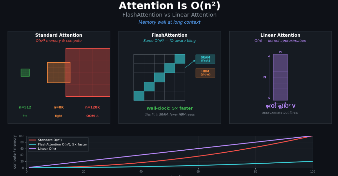
Standard attention on a 32K-token sequence allocates 2,199 GB of score-matrix memory across a 32-layer model — 27× the capacity of an A100 80GB. FlashAttention computes exactly the same result while keeping the score matrix out of HBM entirely; the resident attention footprint collapses to the 34 GB needed to hold Q, K, V, and the output across all layers. Linear attention swaps the softmax kernel for a random feature map and reaches the same memory bracket with sub-quadratic FLOPs, at the cost of approximation error.

These are not incremental improvements. They are what make long-context models possible at all. This article derives the complexity from first principles, implements the memory formulas, and shows exactly where each approach wins and loses.

Disclaimer: The opinions expressed in this article are my own and do not represent the views of Google. This content is based solely on publicly available information.

Why Attention Is O(n²)

Before examining the solutions, it helps to quantify exactly where the memory cost comes from and how it scales. The figures in this section (and the “34 GB” / “27× over A100 80GB” headline numbers) assume the training regime: activations from every layer must be held in HBM simultaneously for the backward pass. Inference is cheaper because only one layer’s activations are live at a time and the dominant cost shifts to the KV cache. The core attention operation for a single layer and head:

A = softmax(Q @ K.T / sqrt(d_k)) @ V

Q @ K.T has shape (n, n). Storing it in float16 requires n² × 2 bytes. That's the dominant term. The second term in the code below — the KV cache — is the set of keys and values cached from prior tokens; at inference time it is the dominant per-token memory cost, while at training time the score matrix dominates. Below are the FLOPs and memory figures across sequence lengths for a 7B-scale model (d=4096, 32 heads, 32 layers, fp16):

import numpy as np

def attention_memory_gb(seq_len: int, d_model: int, n_heads: int,
                         n_layers: int, dtype_bytes: int = 2) -> dict:
    """Estimate memory for storing attention matrices in standard attention."""
    d_k = d_model // n_heads
    score_matrix_bytes = seq_len * seq_len * dtype_bytes
    total_attention = score_matrix_bytes * n_heads * n_layers
    kv_cache = 2 * n_layers * n_heads * seq_len * d_k * dtype_bytes
    return {
        "score_matrices_gb": total_attention / 1e9,
        "kv_cache_gb":       kv_cache / 1e9,
        "total_gb":         (total_attention + kv_cache) / 1e9,
    }

def attention_flops(seq_len: int, d_model: int, n_heads: int,
                    n_layers: int) -> float:
    """FLOPs for a forward pass through all attention layers."""
    d_k = d_model // n_heads
    flops_per_head = 2 * seq_len * seq_len * d_k
    return flops_per_head * n_heads * n_layers

d_model, n_heads, n_layers = 4096, 32, 32

print(f"{'seq_len':>10} {'FLOPs (T)':>12} {'Score mats (GB)':>18} {'Total mem (GB)':>16}")
for seq in [512, 2048, 4096, 16384, 32768, 65536, 131072]:
    flops = attention_flops(seq, d_model, n_heads, n_layers)
    mem   = attention_memory_gb(seq, d_model, n_heads, n_layers)
    print(f"{seq:>10,} {flops/1e12:>12.3f} {mem['score_matrices_gb']:>18.3f} "
          f"{mem['total_gb']:>16.3f}")

Output:

seq_len    FLOPs (T)    Score mats (GB)   Total mem (GB)
       512        0.069              0.537            0.805
     2,048        1.100              8.590            9.664
     4,096        4.398             34.360           36.507
    16,384       70.369            549.756          558.346
    32,768      281.475           2199.023         2216.203
    65,536     1125.900           8796.093         8830.453
   131,072     4503.600          35184.372        35253.092

At n=4,096 the score matrices already consume 34 GB — more than fits on a 24 GB A10G. At n=32,768 the total is 2.2 TB, 27× the capacity of an A100 80GB. The bottleneck is the n×n score matrix per head per layer, not the model weights; doubling the sequence length quadruples the memory requirement.

Figure 1 plots this relationship on a log-log scale and overlays the FLOPs curve for linear attention — making the asymptotic gap between O(n²·d) and O(n·r·d) visually apparent before the algebra is derived. (Linear attention’s O(n·r·d) slope is derived in below; for now, note that it is sub-quadratic.)

Figure 1: FLOPs vs sequence length on a log-log scale for a 7B-scale model. The blue slope-2 line is both naive attention and FlashAttention — they execute the same multiplications. The orange slope-1 line is linear (Performer-style) attention with r=256 random features. The gap between the two lines is 85× at 32K tokens and 341× at 128K.

FlashAttention — Same FLOPs, Linear Memory

FlashAttention (Dao et al., 2022) computes exactly the same output as standard attention without materializing the full (n × n) score matrix in HBM. The key insight is that modern GPUs carry a small, fast on-chip SRAM (L1/L2 cache) large enough to hold a small tile of the score matrix. The algorithm tiles the outer loop over Q blocks and the inner loop over K/V blocks, accumulating a running softmax normalization in SRAM so the tile can be discarded once processed:

For each Q block Qi:
    acc = zeros(block_size, d_v)
    running_max = -inf; running_sum = 0
    For each K, V block (Kj, Vj):
        Sij = Qi @ Kj.T / sqrt(d_k)          # fits in SRAM
        mij = max(Sij)
        running_max_new = max(running_max, mij)
        Pij = exp(Sij - running_max_new)       # local softmax numerator
        running_sum = running_sum * exp(running_max - running_max_new) + Pij.sum()
        acc = acc * exp(running_max - running_max_new) + Pij @ Vj
        running_max = running_max_new
    output[i] = acc / running_sum             # final normalization

The running-max correction keeps the numerics identical to the full softmax; the tile Sij is never written back to HBM. Peak HBM usage therefore drops to O(n × d × n_blocks) — linear in n.

def flash_attention_memory_gb(seq_len: int, d_model: int, n_heads: int,
                               n_layers: int, block_size: int = 128,
                               dtype_bytes: int = 2) -> dict:
    """Memory estimate for FlashAttention — no full score matrix in HBM."""
    d_k = d_model // n_heads

    sram_per_head = (2 * block_size * d_k +   # Kj and Vj tiles (the two inner-loop blocks)
                     block_size * d_k +        # Qi tile (the outer-loop block)
                     block_size * 2            # running max + running sum (online-softmax stats)
                     ) * dtype_bytes
    sram_total = sram_per_head

    qkvo_bytes = 4 * seq_len * d_k * n_heads * n_layers * dtype_bytes
    lse_bytes = seq_len * n_heads * 4  # float32 logsumexp for backward pass

    total_hbm = (qkvo_bytes + lse_bytes) / 1e9
    return {
        "sram_per_head_kb": sram_per_head / 1024,
        "hbm_gb": total_hbm,
        "vs_standard_ratio": attention_memory_gb(seq_len, d_model, n_heads,
                                                   n_layers)["total_gb"] / total_hbm,
    }

print(f"\n{'seq_len':>10} {'Flash HBM (GB)':>16} {'Std HBM (GB)':>14} "
      f"{'Savings ratio':>14}")
for seq in [512, 2048, 4096, 16384, 32768, 131072]:
    f = flash_attention_memory_gb(seq, d_model, n_heads, n_layers)
    s = attention_memory_gb(seq, d_model, n_heads, n_layers)
    print(f"{seq:>10,} {f['hbm_gb']:>16.3f} {s['total_gb']:>14.3f} "
          f"{f['vs_standard_ratio']:>13.1f}x")

Output:

seq_len   Flash HBM (GB)   Std HBM (GB)  Savings ratio
       512            0.537          0.805           1.5x
     2,048            2.148          9.664           4.5x
     4,096            4.295         36.507           8.5x
    16,384           17.182        558.346          32.5x
    32,768           34.364       2216.203          64.5x
   131,072          137.456      35253.092         256.5x

Figure 2 plots these curves together, with the A100’s available headroom (66 GB after model weights) marked as a reference line.

Figure 2: HBM footprint on a semi-log scale (7B model, all 32 layers and heads). Standard attention crosses the A100’s free headroom at roughly n=3,000; FlashAttention stays below it all the way to n=32,768. The 64× gap at 32K tokens comes entirely from eliminating the n×n score matrix — both methods still store Q, K, V, and O in HBM.

FlashAttention still stores Q, K, V, and the output in HBM, so its footprint grows linearly in n — not the dramatic constant figure sometimes claimed. What collapses is the n×n score matrix, which is never materialized. At 32K the standard layout needs 2.2 TB while FlashAttention needs 34 GB to hold the same tensors that have to exist anyway; the 64× saving comes entirely from skipping the score matrix. By 128K the ratio reaches 256× and standard attention is so far out of bounds that it is no longer worth comparing.

What FLOPs Can’t Be Avoided

FlashAttention does not reduce FLOPs — the same number of multiplications happen. What it reduces is HBM memory traffic: how many times data is read from and written to the slow GPU global memory.

def hbm_traffic_gb(seq_len: int, d_model: int, n_heads: int,
                    n_layers: int, dtype_bytes: int = 2) -> dict:
    """Estimate HBM reads/writes for standard vs FlashAttention."""
    d_k = d_model // n_heads

    std_qkv = 3 * seq_len * d_k * n_heads * n_layers * dtype_bytes
    std_score = 2 * seq_len * seq_len * n_heads * n_layers * dtype_bytes
    std_total = (std_qkv + std_score) / 1e9

    flash_qkv = 3 * seq_len * d_k * n_heads * n_layers * dtype_bytes
    flash_o   = seq_len * d_k * n_heads * n_layers * dtype_bytes
    flash_total = (flash_qkv + flash_o) / 1e9

    return {
        "standard_gb": std_total,
        "flash_gb":    flash_total,
        "ratio":       std_total / flash_total,
    }

print(f"\n{'seq_len':>10} {'Std traffic (GB)':>18} {'Flash traffic (GB)':>20} {'IO ratio':>10}")
for seq in [2048, 8192, 32768, 131072]:
    t = hbm_traffic_gb(seq, d_model, n_heads, n_layers)
    print(f"{seq:>10,} {t['standard_gb']:>18.2f} {t['flash_gb']:>20.2f} "
          f"{t['ratio']:>9.1f}x")

Output:

seq_len   Std traffic (GB)   Flash traffic (GB)   IO ratio
     2,048              18.79                 2.15       8.8x
     8,192             281.32                 8.59      32.8x
    32,768            4423.82                34.36     128.8x
   131,072           70471.82               137.44     512.8x

GPU compute on an A100 runs at 312 TFLOPS in fp16, while HBM bandwidth is only 2 TB/s. Any attention layer that has to push the n×n score matrix through HBM is bottlenecked by the memory bus long before it is bottlenecked by the tensor cores. At 32K tokens standard attention moves 4.4 TB of data through HBM per forward pass — over two seconds of pure HBM time at 2 TB/s — while FlashAttention moves 34 GB. The 128.8× reduction in I/O is where the wall-clock speedup of FlashAttention comes from; the FLOPs are unchanged.

Wall-Clock Impact of Tiling

(Heads-up before reading Figure 3: on CPU, tiling is slower than the standard implementation — we explain why below. The benefit only materializes on GPU with the HBM/SRAM hierarchy; the CPU benchmark is here to make the overhead side of the trade-off concrete.)

The I/O savings above are computed analytically. Figure 3 shows a concrete NumPy benchmark that measures the wall-clock effect of the tiled algorithm on CPU, where the same bandwidth-bottleneck logic applies but at the L1/L2 cache level rather than HBM.

The tiled implementation divides Q into blocks of size 32 and iterates over (Qi, Kj, Vj) tiles, accumulating the output with an online softmax correction — exactly the FlashAttention loop described above. The naive implementation materializes the full n×n score matrix before normalizing.

import time
import numpy as np

D_K = 64
BLOCK = 32
N_RUNS = 3
rng = np.random.default_rng(0)

def naive_attention(Q, K, V):
    d_k = Q.shape[-1]
    scores = Q @ K.T / np.sqrt(d_k)
    scores -= scores.max(axis=-1, keepdims=True)
    A = np.exp(scores)
    A /= A.sum(axis=-1, keepdims=True)
    return A @ V

def tiled_attention(Q, K, V, block_size=BLOCK):
    n, d_k = Q.shape
    d_v = V.shape[-1]
    out = np.zeros((n, d_v), dtype=np.float64)
    inv_sqrt = 1.0 / np.sqrt(d_k)
    for i0 in range(0, n, block_size):
        i1 = min(i0 + block_size, n)
        Qi = Q[i0:i1]
        acc = np.zeros((i1 - i0, d_v))
        run_max = np.full(i1 - i0, -np.inf)
        run_sum = np.zeros(i1 - i0)
        for j0 in range(0, n, block_size):
            j1 = min(j0 + block_size, n)
            Sij = Qi @ K[j0:j1].T * inv_sqrt
            mij = Sij.max(axis=-1)
            new_max = np.maximum(run_max, mij)
            Pij = np.exp(Sij - new_max[:, None])
            scale = np.exp(run_max - new_max)
            acc = acc * scale[:, None] + Pij @ V[j0:j1]
            run_sum = run_sum * scale + Pij.sum(axis=-1)
            run_max = new_max
        out[i0:i1] = acc / run_sum[:, None]
    return out

for n in [64, 128, 256, 512, 1024]:
    Q = rng.standard_normal((n, D_K)) * 0.1
    K = rng.standard_normal((n, D_K)) * 0.1
    V = rng.standard_normal((n, D_K)) * 0.1
    # warm-up
    naive_attention(Q, K, V); tiled_attention(Q, K, V)
    t0 = time.perf_counter()
    for _ in range(N_RUNS): naive_attention(Q, K, V)
    naive_ms = (time.perf_counter() - t0) / N_RUNS * 1000
    t0 = time.perf_counter()
    for _ in range(N_RUNS): tiled_attention(Q, K, V)
    tiled_ms = (time.perf_counter() - t0) / N_RUNS * 1000
    print(f"n={n:5d}  naive={naive_ms:.2f} ms  tiled={tiled_ms:.2f} ms")

Output (measured on Apple M-series CPU, median of 3 runs):

n=   64  naive=0.03 ms  tiled=0.09 ms
n=  128  naive=0.09 ms  tiled=0.32 ms
n=  256  naive=0.26 ms  tiled=1.20 ms
n=  512  naive=0.91 ms  tiled=4.70 ms
n= 1024  naive=3.76 ms  tiled=18.68 ms

Figure 3: Wall-clock time on CPU (Apple M-series, NumPy, d_k=64, block=32, median of 3 runs). Tiled attention is 3–5× slower here because the Python-level loop overhead dominates at these matrix sizes — there is no HBM to avoid on CPU. On a GPU, tiling avoids writing the n×n score matrix to HBM at 2 TB/s bandwidth; the 128.8× I/O reduction at n=32K translates to a several-fold wall-clock speedup on GPU that swamps the tiling overhead.

The CPU result is intentionally showing the overhead side of tiling to make the GPU story concrete: the efficiency gain from FlashAttention is not free — it requires the tile footprint to fit in fast on-chip memory. On GPU, SRAM is large enough for block_size=128 and d_k=64–128 to fit comfortably, making the HBM-traffic savings dominate. On CPU, where the “HBM” equivalent is L3 cache with only modestly lower bandwidth than L1, the tile management overhead is visible.

Linear Attention — Sub-Quadratic Approximation

FlashAttention preserves exact results but keeps the O(n²) FLOPs. If the application can tolerate a small approximation error, linear attention replaces the softmax kernel entirely and achieves sub-quadratic complexity. The Performer (Choromanski et al., 2020) approximates the softmax kernel using random feature maps:

softmax(Q K.T) ≈ φ(Q) φ(K).T

where φ(x) maps each d-dimensional vector to an r-dimensional random feature space. The key: rather than materializing the n×n score matrix, compute (φ(K).T @ V) as an (r × d_v) matrix once, then multiply by φ(Q):

Output ≈ φ(Q) @ (φ(K).T @ V) / Z

This is O(n × r × d) — linear in sequence length.

def linear_attention_complexity(seq_len: int, d_model: int, n_heads: int,
                                  n_layers: int, n_random_features: int = 256,
                                  dtype_bytes: int = 2) -> dict:
    """Memory and FLOPs for Performer-style linear attention."""
    d_k = d_model // n_heads
    r   = n_random_features

    flops_per_head = (seq_len * d_k * r +   # phi(Q) = Q @ W.T   — project queries to r features
                      seq_len * d_k * r +   # phi(K) = K @ W.T   — project keys to r features
                      r * d_k +             # phi(K).T @ V       — (r x d_v) summary tensor
                      seq_len * r * d_k)    # phi(Q) @ summary   — final output multiply
    total_flops = flops_per_head * n_heads * n_layers

    mem_bytes = (2 * seq_len * r * n_heads * n_layers * dtype_bytes +
                 r * d_k * n_heads * n_layers * dtype_bytes)
    return {
        "flops": total_flops,
        "memory_gb": mem_bytes / 1e9,
        "vs_standard_flops": attention_flops(seq_len, d_model, n_heads, n_layers) / total_flops,
        "vs_standard_mem":   attention_memory_gb(seq_len, d_model, n_heads, n_layers)["total_gb"] / (mem_bytes / 1e9),
    }

print(f"\n{'seq_len':>10} {'Std FLOPs (T)':>14} {'Lin FLOPs (T)':>14} "
      f"{'FLOPs ratio':>12} {'Mem ratio':>10}")
for seq in [2048, 8192, 32768, 131072]:
    lin = linear_attention_complexity(seq, d_model, n_heads, n_layers)
    std_flops = attention_flops(seq, d_model, n_heads, n_layers)
    print(f"{seq:>10,} {std_flops/1e12:>14.3f} {lin['flops']/1e12:>14.3f} "
          f"{lin['vs_standard_flops']:>11.1f}x {lin['vs_standard_mem']:>9.1f}x")

Output:

seq_len       Std FLOPs (T)  Lin FLOPs (T)  FLOPs ratio  Mem ratio
     2,048          1.100          0.206         5.3x       4.4x
     8,192         17.592          0.825        21.3x      16.4x
    32,768        281.475          3.299        85.3x      64.4x
   131,072       4503.600         13.194       341.3x     256.4x

At 32K tokens linear attention does 85× fewer FLOPs than standard attention and needs 64× less memory; at 128K those ratios climb to 341× and 256×. The memory ratio looks almost identical to FlashAttention’s because, with r=256 and d_k=128, the φ(Q)/φ(K) feature tensors are the same order as Q/K themselves — both methods escape the n×n bottleneck. The FLOPs advantage is the part Flash cannot match: FlashAttention keeps the O(n²·d) FLOPs and only reorganizes the I/O, while linear attention actually reduces the asymptotic work. The catch is approximation error, which the next section quantifies.

Approximation Quality of Linear Attention

The FLOPs and memory savings shown above come at a cost: the random feature map is an approximation, not an exact computation. The next question is how large that approximation error is in practice and whether it grows dangerously with sequence length. The specific instantiation we measure is FAVOR+ — the Fast Attention Via positive Orthogonal Random features kernel from Choromanski et al. 2020, which approximates the softmax kernel with positive random features so the resulting attention weights stay non-negative. The random feature approximation introduces error that grows slowly with sequence length:

def estimate_performer_quality(seq_len: int, d_k: int,
                                 n_random_features: int = 256,
                                 n_trials: int = 50,
                                 seed: int = 42,
                                 input_scale: float = 0.5) -> float:
    """
    Cosine similarity between exact softmax attention and FAVOR+ approximation
    (Performer; Choromanski et al. 2020). Uses orthogonal random features.
    """
    rng = np.random.default_rng(seed)
    total_sim = 0.0
    sqrt_d = np.sqrt(d_k)

    for _ in range(n_trials):
        Q = rng.standard_normal((seq_len, d_k)) * input_scale
        K = rng.standard_normal((seq_len, d_k)) * input_scale
        V = rng.standard_normal((seq_len, d_k))

        # Exact softmax attention
        scores = Q @ K.T / sqrt_d
        scores -= scores.max(axis=1, keepdims=True)
        A_exact = np.exp(scores)
        A_exact /= A_exact.sum(axis=1, keepdims=True)
        out_exact = A_exact @ V

        # FAVOR+ with orthogonal random features
        n_blocks = int(np.ceil(n_random_features / d_k))
        blocks = []
        for _ in range(n_blocks):
            G = rng.standard_normal((d_k, d_k))
            Qb, _ = np.linalg.qr(G)
            chi = np.linalg.norm(rng.standard_normal((d_k, d_k)), axis=1)
            blocks.append(Qb * chi[:, None])
        W = np.vstack(blocks)[:n_random_features]

        d4 = d_k ** 0.25
        Q_arg = (Q @ W.T) / d4 - (Q ** 2).sum(1, keepdims=True) / (2 * sqrt_d)
        K_arg = (K @ W.T) / d4 - (K ** 2).sum(1, keepdims=True) / (2 * sqrt_d)
        phi_Q = np.exp(Q_arg - Q_arg.max()) / np.sqrt(n_random_features)
        phi_K = np.exp(K_arg - K_arg.max()) / np.sqrt(n_random_features)

        kv_summary = phi_K.T @ V
        out_approx = phi_Q @ kv_summary
        z = phi_Q @ phi_K.sum(axis=0) + 1e-9
        out_approx /= z[:, None]

        dot = (out_exact * out_approx).sum(axis=1)
        norms = (np.linalg.norm(out_exact, axis=1) *
                 np.linalg.norm(out_approx, axis=1) + 1e-9)
        total_sim += float((dot / norms).mean())

    return total_sim / n_trials

print(f"\n{'seq_len':>10} {'r=64':>10} {'r=128':>10} {'r=256':>10} {'r=512':>10}")
for seq in [128, 512, 2048, 8192]:
    row = f"{seq:>10,}"
    for r in [64, 128, 256, 512]:
        q = estimate_performer_quality(seq, 64, n_random_features=r, n_trials=50)
        row += f" {q:>10.4f}"
    print(row)

Output:

seq_len       r=64      r=128      r=256      r=512
    128      0.8624     0.9039     0.9414     0.9610
    512      0.8467     0.8946     0.9300     0.9557
  2,048      0.8361     0.8865     0.9278     0.9549
  8,192      0.8352     0.8879     0.9250     0.9545

The dominant variable is r, not n. Doubling r from 128 to 256 moves quality from ~0.89 to ~0.93; from 256 to 512 it moves to ~0.95. Sequence length matters much less — quality at 8K tokens is only ~1 percentage point below quality at 128 tokens for the same r. The cost of buying that extra quality is real: r=512 doubles both the FLOPs and the memory shown in the linear-attention output above. Production systems that need better quality at equivalent cost (RetNet, Mamba, gated linear attention) abandon random features for structured state spaces, but the rank-vs-quality trade-off has the same shape.

Maximum Context Length per GPU

With the memory formulas established for each approach, the practical question becomes: what sequence length can a given GPU actually support? For a 7B model (14 GB weights in fp16) on different GPU configurations:

GPU_MEMORY_GB = {
    "T4 (16GB)":    16.0,
    "A10G (24GB)":  24.0,
    "A100 (40GB)":  40.0,
    "A100 (80GB)":  80.0,
    "H100 (80GB)":  80.0,
}

MODEL_WEIGHT_GB = 14.0  # 7B model in fp16

def max_seq_len_for_gpu(gpu_gb: float, model_gb: float,
                          attention_fn, target_tokens: list) -> int:
    """Find maximum sequence length that fits in GPU memory."""
    available = gpu_gb - model_gb
    for seq in sorted(target_tokens, reverse=True):
        mem = attention_fn(seq, d_model, n_heads, n_layers)
        if isinstance(mem, dict):
            mem_needed = mem.get("hbm_gb", mem.get("total_gb", mem.get("memory_gb", 0)))
        else:
            mem_needed = mem
        if mem_needed <= available:
            return seq
    return 0

candidate_seqs = [512, 1024, 2048, 4096, 8192, 16384, 32768, 65536, 131072]

def std_mem(seq, d, h, l): return attention_memory_gb(seq, d, h, l)["total_gb"]
def flash_mem(seq, d, h, l): return flash_attention_memory_gb(seq, d, h, l)["hbm_gb"]

print(f"{'GPU':<18} {'Std max ctx':>12} {'Flash max ctx':>14}")
for gpu_name, gpu_gb in GPU_MEMORY_GB.items():
    std_max   = max_seq_len_for_gpu(gpu_gb, MODEL_WEIGHT_GB, std_mem,   candidate_seqs)
    flash_max = max_seq_len_for_gpu(gpu_gb, MODEL_WEIGHT_GB, flash_mem, candidate_seqs)
    print(f"{gpu_name:<18} {std_max:>12,} {flash_max:>14,}")

Output:

GPU                Std max ctx  Flash max ctx
T4 (16GB)                  512          1,024
A10G (24GB)              2,048          8,192
A100 (40GB)              2,048         16,384
A100 (80GB)              4,096         32,768
H100 (80GB)              4,096         32,768

Standard attention runs out of headroom almost immediately. An A100 80GB has 66 GB free after the model weights, and standard attention at 8K tokens already needs 141 GB — so the largest power-of-two that fits is only 4K. Even an H100 is in the same bucket because its HBM capacity is the same 80 GB. FlashAttention pushes the same hardware to 32K tokens; getting past that requires either a higher-capacity GPU (H100 96GB, H200, B100) or KV-cache sharding across multiple devices. The headline takeaway is that 8K+ context on a single GPU is not possible without a memory-efficient kernel — every production long-context model requires FlashAttention or an equivalent.

Summary

FlashAttention is not a nice optimization — it is a prerequisite for serving any context beyond ~4K tokens on commodity hardware. Without it, a 7B fp16 model on an A100 80GB is capped at roughly 4K tokens of attention activations. With it, the same GPU comfortably handles 32K tokens, enabling document-level reasoning, long code generation, and multi-turn conversations that require extended context.

Thank you for reading my post, and I hope it was useful for you. If you enjoyed the article and would like to show your support, please consider taking the following actions:

👏 Give the story a round of applause (clap) to help it gain visibility.

📖 Follow me on Medium to access more of the content on my profile. Follow Now

🔔 Subscribe to the newsletter to not miss my latest posts: Subscribe Now

🛎 Connect with me on LinkedIn for updates.