Makemore: Your First Step into Building Language Models (part 1)

In this blog, we will explore how to create a unique name using Makemore. This blog is a note for the video created by Andrej Karpathy (link).

Have you ever wondered how machines can generate human-like text, or even create a unique name that sounds real? Today, we’re diving into Makemore, a project designed to teach you the fundamentals of language modeling step-by-step. Our initial focus will be on generating new, unique names based on a dataset of 32,000 existing names.

1. What is a Character-Level Language Model?

2. How to build a Character-Level Language Model with Makemore?

Makemore operates as a character-level language model → processes and generates text one character at a time, learning the statistical relationships between consecutive characters.

This project is a stepping stone, aiming to eventually progress from character-level to word-level models for document generation, and even advanced image-text networks like DALL-E and Stable Diffusion, with the ultimate goal of building a transformer model equivalent to GPT-2.

2. How to build a Character-Level Language Model with Makemore?

The simplest foundation language model in Makemore is the bi-gram language model. This model predicts the next character by only considering the single character immediately preceding it.

2.1. Build Bi-gram Language Model (Count-Based Approach)

Prepare Your Data with Bi-grams:

• Each word provides multiple bi-gram examples. For instance, for “emma”, “e” followed by “m”, “m” followed by “m”, and so on.
• To capture word beginnings and endings, a special “start” token (.) precedes the first character, and an “end” token (.) follows the last character. For “emma”, the bi-gram would be (., e), (e, m), (m, m), (m, a), (a, .)

Count Bi-gram Occurrences:

• The simplest way to implement a bi-gram model is by counting. You iterate through all the words and extract every consecutive character pair (bi-gram).
• You will need to store these counts. Here, we use a 2D PyTorch array (N). This array has a shape of (27, 27), representing 26 alphabet characters and 1 special start/ end token. Each cell N[row, column] stores how many times the character represented by row is followed by the character represented by column.

# Read the dataset
words = open("names.txt", "r").read().splitlines()

# Create 2D array to hold the bigram counts
N = torch.zeros((27, 27), dtype=torch.int32)

# Extract all unique characters in words, and sort them
chars = sorted(list(set(''.join(words))))
# string to integer -> map each character to a unique integer index
stoi = {c: i+1 for i, c in enumerate(chars)}
# map character '.' to 0
stoi['.'] = 0
# integer to string -> reverse mapping: convert integer back to character
itos = {i: c for c, i in stoi.items()}

for w in words:
 # Add start (.) and end (.) tokens to the word
  chs = ['.'] + list(w) + ['.']
  for ch1, ch2 in zip(chs, chs[1:]):  # Iterate through all bigrams
      i1 = stoi[ch1]  # Convert ch1 to its index
      i2 = stoi[ch2]  # Convert ch2 to its index
      N[i1, i2] += 1  # Increase the count for this bigram in the matrix

We can visualize the counts using code below:

import matplotlib.pyplot as plt
%matplotlib inline

plt.figure(figsize=(16, 16))
plt.imshow(N, cmap='Blues')
for i in range(27):
    for j in range(27):
        chstr = itos[i] + itos[j]
        plt.text(j, i, chstr, ha='center', va='bottom', color='black')
        plt.text(j, i, N[i, j].item(), ha='center', va='top', color='black')

plt.axis('off')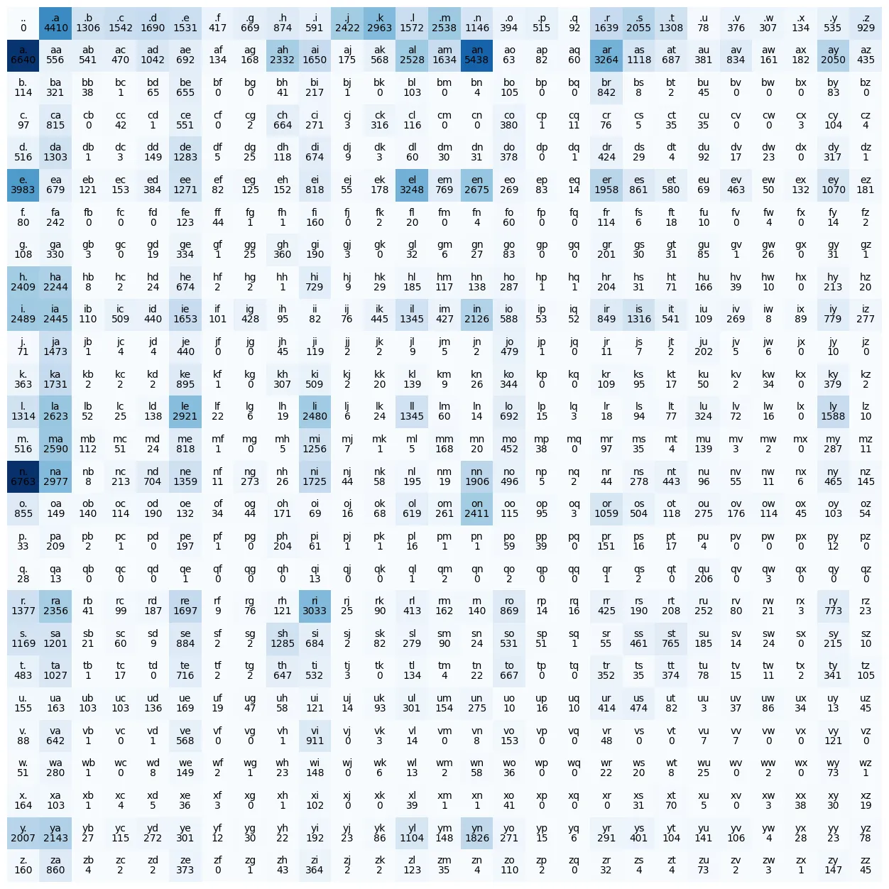

As can be seen from the count matrix, the bigram “aa” exists 4410 times in the dataset, etc.

Normalize Counts to Probabilities:

• Once you have the raw counts, you need to normalize them to create probability distributions. For any character, the probability of that character is done by dividing the count of each bi-gram by the total count of all bi-grams starting with that character.

P = N.float()
P /= P.sum(dim=1, keepdim=True)  # normalize each row

Note: Broadcasting in PyTorch

Broadcasting determines whether two tensors can be combined in a binary operation (such as +, -, *, /) even if their shapes are not the same.

Broadcasting rule:

• Each tensor has at least one dimension
• When iterating over the dimension sizes, starting at the trailing (rightmost) dimension, the dimension sizes must either be equal, one of them is 1, or one of them does not exist

P                           
-> (27,27)
P.sum(dim=1, keepdim=True)  
-> (27,1) -> (27,27)  
-> replicated horizontally

# The importance of keepdim=True
P.sum(dim=1, keepdim=False) 
-> (27) -> (1,27) -> (27,27) 
-> replicated vertically 
-> different output although the operation being broadcasting

2.2. Generate Name from Bi-gram Model (Sampling)

With the probabilities (P matrix) established, your model can now generate new names.

# Generate 10 sample names
for i in range(10):
    out = []
    # Start with the special start token (index 0)
    idx = 0
    while True:
        p = N[idx].float()
        p = p / p.sum()
        # Sample next character index from p probability distribution
        idx = torch.multinomial(p, num_samples=1, replacement=True, generator=g).item()
        # Convert index back to character and add to output
        out.append(itos[idx])
        # If end token is generated, stop
        if idx == 0:
            break
    print(''.join(out))

The output will be something like below.

It’s worth noting that this simple bi-gram model often generates terrible or “nonsense names” because it only considers the immediate preceding character, “forgetting the fact that we may have a lot more information”.

2.3. Evaluating Model Quality with Negative Log Likelihood (NLL)

To understand how “good” your model is, we need a loss function.

Likelihood: The quality of the model is measured by its likelihood, which is “the product of all of these probabilities”.

Log-Likelihood:

• Using Likelihood, the quality is easily becoming extremely small (products of many probabilities between 0 and 1) :

P(sequence) = P(w₁) × P(w₂|w₁) × P(w₃|w₁,w₂)

• To avoid this, we convert products into sums, using the log-likelihood:

log P(sequence) = log P(w₁) + log P(w₂|w₁) + log P(w₃|w₁,w₂)

→ Log-likelihood is just “the sum of the logs of the individual probabilities.”

Negative Log-Likelihood (NLL) Loss: Since log-likelihood is always a negative number, to create a loss function where “low is good,” we take the negative of the log-likelihood.

• Goal: find the parameters that minimize the negative log likelihood loss
• A lower NLL indicates that the model assigns higher probabilities to the correct next characters in the training data. The average NLL over all training examples is the final loss value.

log_likelihood = 0.0
n = 0
for w in words:
    chs = ['.'] + list(w) + ['.']
    for ch1, ch2 in zip(chs, chs[1:]):
        i1 = stoi[ch1]
        i2 = stoi[ch2]
        prob = P[i1, i2]
        logprob = torch.log(prob)
        log_likelihood += logprob
        n += 1
        # print(f'{ch1}{ch2}: {prob:.4f} {logprob:.4f}')
print(f'Log likelihood: {log_likelihood:.4f}')
nll = -log_likelihood
print(f'Negative log likelihood: {nll:.4f}')
print(f'Average negative log likelihood: {nll / n:.4f}')
-------
Log likelihood: -559891.7500
Negative log likelihood: 559891.7500
Average negative log likelihood: 2.4541

2.4. Neural Network Approach to Bi-gram Language Modeling

Disadvantages of Bi-gram:

• While counting works for simple bi-grams, it becomes infeasible for longer sequences because the “tables would get way too large” due to ca ombinatorial explosion.
• For example, for a bi-gram, you have 27 (possible previous characters) 27 (possible next characters) entries in your table. If you want to consider trigrams (predicting the next character based on the two previous characters), you’d need a table of 27 27 * 27 entries. If you wanted to consider the last 10 characters, the table size would become 27 raised to the power of 10.

→ unscalable for learning complex, long-range dependencies in language.

→ Neural Network Approach

Advantages of NN:

• When you go below for NN, you can see that NN is more scalability and flexibility. While counting becomes impractical for longer sequences (e.g., considering the last 10 characters), NN can handle complex relationships and larger contexts without explicitly storing every combination in a massive table.

Create Training Set (Inputs and Targets):

• Just like before, you’ll create pairs of (input character, target next character) from your dataset.

# Create the training set of bigrams (x, y)
xs, ys = [], []

for w in words[:1]:
    chs = ['.'] + list(w) + ['.']
    for ch1, ch2 in zip(chs, chs[1:]):
        i1 = stoi[ch1]
        i2 = stoi[ch2]
        xs.append(i1)
        ys.append(i2)
xs = torch.tensor(xs)
ys = torch.tensor(ys)

One-Hot Encode Inputs:

• Neural networks can’t directly process integer indices. Instead, you transform them into one-hot encoded vectors.
• For example, if ‘a’ is index 0 and ‘b’ is index 1, ‘a’ would become [1, 0, 0, …, 0] and ‘b’ would be [0, 1, 0, …, 0]

import torch.nn.functional as F
xenc = F.one_hot(xs, num_classes=27).float()

Single-Layer Neural Network (Weights and Logits):

• Your network will start with a single linear layer, represented by a weight matrix W (also 27x27). This matrix is initially filled with random numbers.
• The one-hot encoded inputs are multiplied by W (x_enc @ W). The output of this multiplication are raw "firing rates" called logits. These logits are essentially interpreted as "log counts".

W = torch.randn((27, 27))
xenc @ W

Get Probabilities for log counts:

• To convert these logits into proper probability distributions (positive numbers that sum to one), exponentiates the logits to get “fake counts” and then normalizes them across each row to sum to 1, creating a probability distribution for each input example.

logits = xenc @ W # log counts
counts = logits.exp()   # counts, equivalent to N
probs = counts / counts.sum(dim=1, keepdim=True) # probabilities for next character

Calculate Loss (NLL):

• For each input example, the model’s probability for the correct next character is extracted from the probs matrix, log-transformed, negated, and averaged to get the final loss value.

loss = -probs[torch.arange(5), ys].log().mean()

Optimize with Gradient Descent:

# backward pass
W.grad = None    # Reset gradients for W to zero
loss.backward()  # Compute gradients of the loss with respect to all parameters

# update
W.data += -learning_rate * W.grad  # Adjust the weights W in the opposite direction of their gradients to minimize the loss 

Iteration: Repeat the above steps (from Single-Layer Neural Network (Weights and Logits)) for many epochs

• This is the full code:

for k in range(10):
    # forward pass
    xenc = F.one_hot(xs, num_classes=27).float()
    logits = xenc @ W
    counts = logits.exp()   # counts, equivalent to N
    probs = counts / counts.sum(dim=1, keepdim=True) # probabilities for next
    loss = -probs[torch.arange(num), ys].log().mean()
    print(loss.item())

    # backward pass
    W.grad = None
    loss.backward()

    # update
    W.data += -0.1 * W.grad

You can check my repo at the link:

https://github.com/chautuankien/Makemore

References:

• Andrej Karpathy’s Makemore Video