Heterogeneous Effects, Uplift, and Bandits: From Average Treatment Effects to Individualized Decisions

Part 6 of 7. Personalizing treatment and learning policies online.

This is the sixth article of a seven-part series on Bayesian methods in industry. Part 1 covered the foundations of Bayesian thinking. Part 2 covered the computational machinery. Part 3 covered hierarchical models and GLMs. Part 4 covered Bayesian Marketing Mix Modeling. Part 5 covered classical causal inference and debiased machine learning. Part 7 covers Bayesian Deep Learning, Gaussian Processes, and Bayesian Optimization.

The Thesis

The previous article ended with the average treatment effect. The ATE is the right answer to a specific class of questions: “should we deploy this intervention to the population as a whole.” It is the wrong answer to a much larger class of questions, which are about individuals. Whether to send a retention offer to this customer. What price to quote this user. Which creative variation to show this visitor. Which dose to recommend to this patient.

A positive ATE can mask groups for whom the effect is zero, negative, or large enough to dominate the average. Personalizing the decision requires the conditional average treatment effect, the policy that maps individual features to optimal treatments, and a methodology for learning that policy online when the right action is not known in advance.

The shift from ATE to CATE changes the questions you can answer and the methods that answer them. Causal Forests (Athey, Wager, Tibshirani 2019), CausalForestDML (EconML), and the meta-learner family (Künzel et al. 2017) are the workhorses for CATE estimation. Uplift modeling reframes the problem in marketing-friendly language with quadrants of persuadable, sure-thing, lost-cause, and do-not-disturb customers. Policy learning translates the CATE into an action recommendation, with cost awareness baked in. And bandits provide the framework for learning the right action when you have to decide repeatedly and can observe the consequences.

This is the most operationally consequential article in the series. The methods covered here are what drive the difference between a model that estimates effects and a system that takes actions. The core libraries (EconML, CausalML, Vowpal Wabbit, Open Bandit Pipeline) are mature enough for production use in expert teams, though some advanced variants (conformal CATE, federated causal learning, Bayesian RL, advanced BOCD, Bayesian active learning at frontier scale) remain research-grade and need expertise to deploy safely. The patterns are stable. And the cases (personalized pricing, real-time budget allocation, uplift-driven retention) are where Bayesian and ML-causal methods produce measurable business value.

Part I. Why the ATE Is Not Enough

The average treatment effect averages over the population. The mean might be positive while large subgroups have effects of zero or negative. The two failure modes of acting on the ATE are well-known.

Treating everyone when only some respond. A retention offer with positive ATE may include large groups for whom the offer has no effect or a negative effect. The persuadables (who respond positively) drive the average; the sure-things (who would have stayed anyway), the lost-causes (who leave regardless), and the do-not-disturbs (who are pushed away by the offer) all dilute or counteract the persuadable effect. Treating everyone wastes budget on customers who would have stayed and creates churn among customers the offer alienates.

Failing to treat when the average is small but pockets are large. A pricing test may have a small ATE because high-income customers are insensitive and low-income customers are highly sensitive in opposite directions. Reporting a single number obscures the heterogeneity that determines the right pricing strategy.

The CATE addresses both. The conditional average treatment effect τ(x) = E[Y(1) — Y(0) | X = x] is the treatment effect for individuals with features x. With a good CATE estimate, you can identify who responds positively, who responds negatively, who is indifferent, and design a policy that acts accordingly.

The challenge is that CATE estimation is harder than ATE estimation. The ATE is a single number; the CATE is a function. Estimating a function from data is statistically more demanding, and the methods need to handle the variance of individual estimates while still extracting the signal.

Part II. Causal Forests

The causal forest (Athey, Wager, Tibshirani 2019) is a random-forest-based estimator for the CATE. It adapts the regression forest to the causal setting through three key modifications.

Honest splits. The data used to choose the splits in a tree are different from the data used to estimate the values in the leaves. The honesty property is essential for valid asymptotic inference: without it, the splits chase noise and the leaf estimates are biased. The original Athey-Wager-Tibshirani construction uses a clean sample-split.

Splits that maximize treatment effect difference. A regression forest splits to maximize the variance of the outcome between leaves. A causal forest splits to maximize the difference in treatment effects between leaves. The objective function is specifically designed for the causal target.

Local treatment effect estimation. Each leaf provides a local estimate of the treatment effect for units that land in it. The forest’s overall CATE estimate is a weighted average of the leaf estimates, with weights determined by which leaves contain points similar to the query point.

The result is an estimator that, under regularity conditions (honesty, sufficient overlap, well-behaved nuisance estimation, adequate sample size, smoothness of the underlying CATE), provides individual CATE estimates with asymptotically valid confidence intervals. The forest scales to large samples and high-dimensional covariates with substantially improved robustness to overfitting relative to naive tree procedures, but it still overfits when overlap is sparse, signal is weak, nuisance estimation is noisy, neighborhoods are too small, or trees are too deep. The inferential guarantees should not be treated as automatic outside the regime where those conditions hold.

The original R implementation is grf (generalized random forests). The closest Python workhorse is econml.dml.CausalForestDML, which combines the causal forest with DML residualization; the two libraries are related in spirit and complementary in API but are not strictly equivalent.

Part III. CausalForestDML and Orthogonal Forests

CausalForestDML combines the DML residualization (Article 5) with the causal forest. The procedure is:

1. Fit nuisance models ĝ(X) = [Y | X] and m̂(X) = [T | X] using arbitrary ML methods, with cross-fitting.

2. Compute residuals Ỹ = Y — ĝ(X) and T̃ = T — m̂(X).

3. Fit a causal forest on the residuals.

The DML step removes the influence of the high-dimensional confounders on the treatment effect estimation. The causal forest then captures the heterogeneity in the residualized treatment effect. The combination is the workhorse for CATE estimation in EconML.

The orthogonal forests (Oprescu, Syrgkanis, Wu 2019) extend this idea with local cross-fitting: at each query point, the nuisance models are refitted on a local neighborhood. This is more expensive but reduces bias when the nuisance functions vary substantially over the feature space. The implementations are DMLOrthoForest and DROrthoForest in EconML.

The choice between CausalForestDML, DMLOrthoForest, and DROrthoForest is mostly a tradeoff between speed and bias. CausalForestDML is faster and is the default for large datasets. The orthogonal forests are slower but reduce bias when the data are heterogeneous in nuisance structure.

Part IV. Meta-Learners

The meta-learner framework (Künzel, Sekhon, Bickel, Yu 2017) decomposes the CATE estimation into standard supervised learning subproblems. Each meta-learner combines ML methods in a different way to estimate τ(x).

S-learner: a single model. Fit f̂(X, T) = [Y | X, T] as a regression of Y on the joint (X, T). The CATE estimate is τ̂(x) = f̂(x, 1) — f̂(x, 0).

The S-learner’s weakness is that the treatment is just one feature among many. If the algorithm regularizes T heavily (because the treatment effect is small relative to the prognostic effect of X), the CATE estimate can be biased toward zero. This is the dominant failure mode for tree-based S-learners.

T-learner: two separate models. Fit ĝ_1(X) = [Y | X, T=1] on the treated subsample and ĝ_0(X) = [Y | X, T=0] on the untreated subsample. The CATE estimate is τ̂(x) = ĝ_1(x) — ĝ_0(x).

The T-learner’s weakness is variance. With small treated or untreated samples, the two models are noisy and their difference is even noisier. The CATE estimate is dominated by sampling variability in the smaller group.

X-learner: imputes the counterfactual and then models the effect. The procedure is:

1. Fit ĝ_1 on treated, ĝ_0 on untreated.

2. Impute counterfactual outcomes for treated using ĝ_0 and for untreated using ĝ_1.

3. Compute imputed treatment effects: τ̃_i = Y_i — ĝ_0(X_i) for treated, τ̃_i = ĝ_1(X_i) — Y_i for untreated.

4. Fit a regression of τ̃ on X, separately for treated and untreated.

5. Average the two regression estimates, weighted by the propensity score.

The X-learner often outperforms the T-learner when the treated and untreated samples are very different in size, although the comparison depends on nuisance quality, overlap, and the severity of the imbalance. It is often a strong default for imbalanced treatment assignment, which is common in observational marketing data where, for example, 5 percent of customers received a particular offer.

R-learner (Nie, Wager 2021): minimizes a residualized loss directly. The R-learner is essentially the DML procedure written as a meta-learner. It enjoys the Neyman orthogonality property and is the most theoretically principled of the meta-learners.

Domain-Adaptation learner: when the treated and untreated distributions differ in covariates (selection bias in observational data), this learner adapts the models using domain adaptation techniques. The right choice when the propensity is extreme in parts of the feature space.

The meta-learners are implemented in EconML (metalearners module) and CausalML. The choice between them is empirical: in practice, X-learner and CausalForestDML often outperform the others, but the right answer depends on the data and is worth testing with cross-validation.

Part V. Dynamic DML for Sequential Treatments

When the treatment is assigned over time and influenced by previous outcomes (an adaptive marketing policy that adjusts based on what worked yesterday), the static DML framework is not enough. The treatments at different times are correlated with each other and with past outcomes, which breaks the standard assumptions.

Dynamic DML (Lewis, Syrgkanis 2020) extends DML to sequential settings. The procedure handles the time structure explicitly, treating the past treatments as part of the conditioning set and applying the Neyman orthogonality framework to each time step.

The implementation is econml.dynamic.dml.DynamicDML. The use cases are dynamic pricing (where each day’s price depends on yesterday’s demand), multi-touch retention (where each retention action depends on prior responses), and any setting where the marketing policy adapts over time within a customer.

Dynamic DML still buys the usual sequential ignorability and overlap assumptions at each time step: it does not solve hidden state, unobserved feedback loops, or omitted time-varying confounders. The procedure is the right tool when the time-varying confounders are observed and the sequential treatment depends on them; it is not a workaround for genuinely unidentified longitudinal effects, where the g-methods of Article 5 (g-formula, IPW, MSM) or longitudinal TMLE are the appropriate frameworks.

Part VI. Uplift Modeling

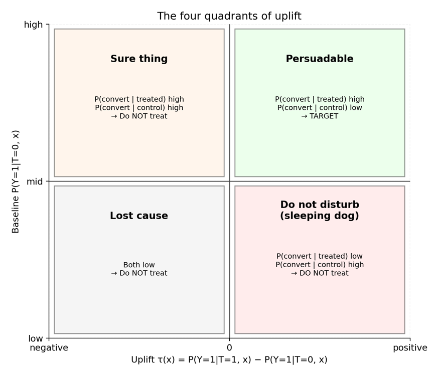
The four uplift quadrants: target persuadables, avoid the rest

Uplift modeling is the marketing-flavored reframing of CATE estimation. The CATE is a continuous function τ(x); the uplift framing categorizes individuals into one of four quadrants based on τ(x) and the baseline outcome under no treatment.

Persuadables: positive treatment effect. They convert (or stay, or buy) only if treated. These are the targets of the marketing action.

Sure things: would convert regardless of treatment, with high probability. The empirical treatment effect is often near zero, sometimes slightly positive (a small reinforcement), sometimes slightly negative (the offer cannibalizes margin or cues attrition). Treatment is mostly wasted on them.

Lost causes: would not convert regardless of treatment. Treatment effect is typically near zero, occasionally slightly positive if the offer reaches a marginal subset. Treatment is mostly wasted on them too.

Do-not-disturbs (sleeping dogs): negative treatment effect. The treatment annoys them or signals something they did not want to notice. They leave because of the treatment, or convert less because of it.

The quadrant framing exposes the key insight: targeting by predicted outcome (the propensity-to-convert model) confuses sure things and lost causes with persuadables. Targeting by predicted uplift correctly identifies persuadables and avoids wasting treatment on the other three quadrants.

The standard uplift modeling pipeline:

1. Run an experiment (or use historical RCT data) with random assignment to treatment and control.

2. Estimate τ(x) using a meta-learner (X-learner or R-learner) or a CausalForest.

3. Sort customers by predicted uplift.

4. Target the top quantile.

5. Validate with a holdout in the next campaign.

The libraries are scikit-uplift (lightweight meta-learners), causalml (Uber’s offering with sensitivity analysis and value optimization), and EconML for the CATE estimation.

Part VII. Cost-Aware Uplift

Naive uplift targeting maximizes total uplift. Production uplift maximizes total value, which accounts for the costs of treatment.

Conversion costs are costs that are paid only when the customer converts. A loyalty discount, for example, is granted only on a purchase. These costs scale with the converted volume.

Impression costs are costs that are paid for every treated customer regardless of outcome. An SMS, an email, a paid ad impression. These costs scale with the treated volume.

The value function combines these:

where v(x) is the value of a conversion (per-customer LTV or transaction value) and c_T(x) is the cost of treatment, which may be a mix of impression and conversion costs.

The optimal policy is to treat each customer whose value function is positive:

In the binary case this reduces to treating customers with τ(x) · v(x) > c_T(x). With multi-level treatments (no offer, small offer, large offer), the policy compares the value across all options and picks the best.

CausalML’s optimize module implements counterfactual value optimization, which directly maximizes the expected value rather than the uplift. The distinction matters operationally: a customer with high uplift but low value (they might convert only on a 10 purchase) is not the right target if treatment costs 5; a customer with moderate uplift and high value is a better target.

Part VIII. Policy Learning

Policy learning is the explicit construction of a function from features to actions. The CATE estimate is a regression on the treatment effect; the policy is a decision rule.

DR Policy Forest (Athey, Wager 2021) is the standard estimator for the optimal policy. The implementation is econml.policy.DRPolicyForest. The approach is:

1. Estimate the doubly robust scores for each treatment-feature combination.

2. Fit a forest that splits the feature space into regions where the optimal treatment is constant.

3. The policy returns the treatment that maximizes the DR score in the region containing the query point.

The output is an interpretable policy tree: at each leaf, a single treatment is recommended. The depth of the tree controls the granularity of the policy, with deeper trees producing more individualized policies at the cost of robustness.

The regret of the learned policy is the expected difference between the value of the learned policy and the value of the optimal policy. Under standard conditions (bounded policy class complexity, overlap, sufficiently fast convergence of the nuisance estimators, and margin or low-noise assumptions where they apply), DR policy learning can achieve strong regret guarantees, in some regimes at near-parametric rates. The exact rate depends on the policy class, the complexity measure used, the nuisance estimation quality, and the margin assumptions; the take-away is that DR policy learning is theoretically grounded, not that it achieves a universal rate.

Part IX. Interpretability of CATE and Policy

A causal forest produces individual CATE estimates. A policy forest produces individual recommendations. Neither is directly interpretable: there is no single coefficient to inspect, no rule to read out.

The standard interpretability tools in EconML are tree-based summaries of the model.

SingleTreeCateInterpreter fits a single shallow decision tree to the CATE estimates produced by any EconML estimator. The splits are chosen to maximize the difference in treatment effect between leaves. With max_depth=2 or max_depth=3, the result is a small tree that exposes the main sources of heterogeneity.

The pattern of use:

from econml.cate_interpreter import SingleTreeCateInterpreter from econml.dml import CausalForestDML

est = CausalForestDML(…) est.fit(Y, T, X=X, W=W)

intrp = SingleTreeCateInterpreter(include_model_uncertainty=True, max_depth=2, min_samples_leaf=10) intrp.interpret(est, X) intrp.plot(feature_names=feature_names)

The output is a plot of the tree, where each leaf shows the estimated treatment effect for the subgroup defined by the path from root to leaf. This is the answer to “where is the heterogeneity”: the features that appear at the top of the tree are the ones that most determine treatment response.

SingleTreePolicyInterpreter is the analogous tool for policy. It fits a shallow tree that splits the feature space into subgroups with different recommended treatments. The output is a decision rule that can be communicated to stakeholders: “treat customers with feature X above threshold Y; do not treat below.”

These tools sacrifice some accuracy in exchange for interpretability. The single shallow tree cannot capture all the heterogeneity the original forest models. But the result is a rule that a business stakeholder can understand, audit, and override when needed.

Part X. Federated Causal Learning

In regulated industries (banking, healthcare, telecoms), data often cannot leave the client environment. Centralized causal modeling is impossible because the data are distributed across nodes that cannot share raw observations.

Federated causal learning is the framework for fitting causal models across distributed nodes without centralizing the data. EconML has federated learning support that aggregates gradients or nuisance estimates rather than raw data, applied to DML and DR-style estimators.

Federated causal learning is promising but still operationally more specialized than centralized DML/DR workflows. The statistical and operational picture depends on heterogeneity across nodes (different distributions, different propensity structures, different treatment regimes), communication frequency, the privacy mechanisms layered on top (secure aggregation, differential privacy), the quality of local nuisance estimation, and overlap viewed globally rather than per-node. The use cases are concentrated in regulated industries where centralization is legally impossible; in less constrained settings, the operational cost of federation usually outweighs the marginal privacy benefit.

Part XI. Model Selection in Causal ML

The classical model selection problem (cross-validate the predictive accuracy) does not apply to causal inference. The right metric is the accuracy of the treatment effect estimate, but the treatment effect is unobserved, so accuracy cannot be directly measured.

The workaround is proxy losses that are valid for CATE selection.

R-loss (Nie, Wager 2021): a residualized loss that equals the squared error of the CATE estimate plus a term that does not depend on the CATE. Minimizing R-loss is equivalent to minimizing squared CATE error.

DR-score: the doubly robust score for a candidate CATE estimate. Provides a cross-validated estimate of the policy value, which is the quantity that ultimately matters for decision quality.

EconML provides econml.score.RScorer and econml.score.DRScorer for these losses. The right practice is to use them for model selection during development.

The independent check is to validate the chosen model against held-out experimental data (a small RCT held out from training). This is the gold-standard validation when it is available.

Part XII. Bandit Theory

Multi-armed bandit problems are the simplest case of online learning under uncertainty. An agent chooses one of K arms, observes a reward, and updates its beliefs about the arm distributions. The objective is to minimize cumulative regret, the difference between the reward of the chosen arms and the reward of always picking the best arm.

The exploration-exploitation tradeoff is the central tension. Exploiting (picking the arm that currently looks best) maximizes immediate reward but risks missing a better arm. Exploring (picking arms that currently look worse) sacrifices immediate reward in exchange for information that may pay off later.

Canonical algorithms

Cumulative regret over time: random vs ε-greedy vs UCB vs Thompson Sampling

Epsilon-greedy picks the best-known arm with probability 1 — ε and a random arm with probability ε. Simple, easy to implement, but produces linear regret if ε is fixed. With ε decaying over time, the regret can be made sublinear but suboptimal.

Optimistic initialization sets the initial reward estimates to high values. The agent picks the arm with the highest current estimate, which drives early exploration. The principle “optimism in the face of uncertainty” underlies several more sophisticated algorithms.

UCB1 (Upper Confidence Bound, Auer, Cesa-Bianchi, Fischer 2002) picks the arm with the highest upper confidence bound on the mean. The bound shrinks as more samples are collected, so well-tested arms with low estimates fall behind and exploration concentrates on arms whose bounds are still wide. UCB1 achieves logarithmic regret.

Bayesian UCB replaces the frequentist confidence bound with a Bayesian credible interval. With a prior on the arm distributions, the upper quantile of the posterior plays the role of the UCB. The advantage is natural incorporation of prior information.

Thompson Sampling (Thompson 1933) maintains a posterior over each arm’s mean and picks the arm with the highest sample drawn from the posterior. The sampling rather than the deterministic UCB produces a kind of probability matching: each arm is picked with probability equal to the posterior probability that it is the best.

Thompson Sampling is often one of the strongest practical defaults across many empirical evaluations. The Chapelle and Li (2011) rediscovery of Thompson Sampling, and the subsequent theoretical analysis (Russo, Van Roy and others), established it as a modern default for many bandit problems. Whether it dominates UCB, ε-greedy with decay, bootstrapped TS, LinUCB, conservative bandits, or contextual methods depends on the structure of the problem (reward distribution, prior quality, non-stationarity, batched feedback, safety constraints), and a head-to-head comparison on the specific setting is part of any serious deployment.

The Beta-Bernoulli case

Thompson Sampling Beta-Bernoulli: posteriors concentrate on the best arm as data accumulate

For binary rewards (click, conversion, success) with a Beta prior, Thompson Sampling is exact and closed-form. The posterior after α successes and β failures is Beta(α + α_0, β + β_0) where α_0, β_0 are the prior parameters. Sampling is a single function call, and the update is incremental.

This is the right starting point for simple stationary binary-reward bandits: lightweight A/B testing, click-through optimization, conversion optimization with i.i.d. rewards. The implementation is small, the math is exact, and the performance is strong in that regime. Production bandits often need additional structure on top (context-aware reward models, handling of delayed and batched feedback, non-stationarity, interference between arms, budget constraints, multiple objectives, safety guardrails), and once those become first-order concerns the right tool is a contextual or conservative variant rather than plain Beta-Bernoulli.

Part XIII. Contextual Bandits

The classical bandit assumes the arms have stationary reward distributions. The contextual bandit allows the reward to depend on a context observed before the action: the user’s features, the time of day, the device, the current state of the world.

LinUCB (Li, Chu, Langford, Schapire 2010, the Yahoo News bandit) assumes the expected reward of each arm is linear in the context: E[r | x, a] = x^T θ_a. The algorithm maintains a posterior over θ_a and uses an upper confidence bound on the predicted reward.

LinUCB is the right baseline for contextual bandits with low-dimensional contexts. It is fast, has theoretical guarantees, and works well when the linearity assumption is approximately satisfied.

Linear Thompson Sampling replaces the UCB with sampling from the posterior of θ_a. Comparable to LinUCB in performance, often simpler to implement.

NeuralUCB and Neural Thompson Sampling replace the linear reward model with a neural network. Appropriate when the linearity assumption is too restrictive. The tradeoff is more compute and less theoretical guarantee.

Neural contextual bandits are an active research area. Recent work (Riquelme, Tucker, Snoek 2018; many others) explores variants with deep representation learning, transfer across arms, and other extensions. In production, the simpler linear or shallow methods often outperform deep variants because the contextual features in many problems are not deeply structured.

Cold start

Cold start is the central challenge in contextual bandits: how do you make good decisions when you have no data on a new arm or in a new context? The standard approaches are:

· Prior incorporation: start with an informative prior derived from offline data or domain knowledge.

· Forced exploration floor: ensure every arm receives some minimum traffic regardless of its current estimate.

· Pre-training: train the model offline on existing data (lift tests, A/B tests, observational) and use that as the initialization.

The neural contextual bandit literature has paid particular attention to cold start, with several recent papers on transfer learning and meta-learning approaches.

Part XIV. Bandit-Based Active Learning

When labeling is expensive (a human annotator, a costly experiment), choosing which examples to label is a sequential decision-making problem. The canonical formulation is acquisition-function optimization: maximize an information-theoretic criterion (BALD, expected error reduction, variance reduction) over candidate examples and label the top-ranked ones. The bandit analogy is partial rather than complete: arms here are candidate examples, the reward is the information gained from labeling, and the explore-exploit tension does exist, but the standard frequentist or Bayesian active learning literature usually treats this as acquisition optimization with diversity penalties rather than as a strict K-armed bandit problem. Bandit framings appear in sequential settings with online feedback and stochastic costs, and in those settings the bandit machinery is more directly applicable.

The use cases are data labeling for ML training, A/B testing where the test allocation is itself optimized, and any expensive measurement problem where the question is which subset to invest in.

Part XV. Bandits Versus A/B Tests

The tradeoff is operational and statistical.

A/B tests keep traffic allocation fixed (typically 50/50) for the duration of the experiment. The advantage is clean statistical inference at the end: a p-value, a confidence interval, a defensible conclusion. The disadvantage is operational regret: during the test, half the traffic goes to the suboptimal arm, which is a cost in revenue, conversion, or whatever the metric is.

Bandits dynamically reallocate traffic toward the better-performing arm. The advantage is reduced operational regret: most of the traffic goes to the better arm once it is identified. The disadvantage is inference complexity: standard confidence intervals and p-values are not valid under adaptive data collection. The data have been chosen in a way that depends on previous outcomes, which violates the i.i.d. assumption of classical inference.

The literature on post-bandit inference (Hadad, Hirshberg, Zhan, Wager, Athey 2021; Zhang, Janson, Murphy 2021) has developed estimators that account for the adaptive data collection. They are more complex than classical inference and require the bandit’s exploration probabilities to be recorded.

The operational rule is:

• A/B test when you need a defensible verdict for a one-time decision (launch or not, ship or not). The clean inference is worth the regret cost.
• Bandit when you make the decision repeatedly (every user, every session, every day) and the cost of the regret accumulates. The adaptive allocation pays off over time.
• Hybrid approaches exist: run a short A/B exploration phase, then switch to bandit-style exploitation. The right tradeoff depends on the cost structure and the expected time horizon.

Part XVI. Case Studies

Case A: Personalized Pricing

The setup. A SaaS company offers tiered pricing. Historical discounts have been applied by sales reps with substantial discretion (larger customers receive larger discounts on average). The company has 2,000 historical customer-deal observations with features (size, industry, tenure, usage) and outcomes (whether the deal closed and at what price).

The question. What is the conditional effect of a discount on conversion probability, heterogeneous in customer features? The policy should specify discount levels per customer that maximize expected revenue.

The decision. CausalForestDML with cross-fitting for the CATE, SingleTreeCateInterpreter for the heterogeneity story, DRPolicyForest with a cost function for the policy.

Why not the alternatives.

• A logistic regression with discount-feature interactions assumes linear heterogeneity. The literature (and the EconML case study) shows that price elasticity is often non-monotonic in customer size: very small customers cannot afford anyway, mid-size customers are highly sensitive, large customers are less price-sensitive. Linear interactions miss this.
• The T-learner is feasible but with 2,000 observations and continuous discount, the per-treatment-level models overfit.
• The X-learner is applicable and worth comparing.
• A causal forest without DML residualization would not handle the confounding (larger customers received more discount) cleanly.
• A randomized experiment would be ideal but the sales team refuses to randomize discount on large deals because of the perceived revenue risk.
• A bandit would come later: first understand the heterogeneity offline, then optionally deploy a bandit to refine the policy online.

Assumptions purchased.

· All confounders that influenced the rep’s discount decision are in the feature set (size, industry, tenure, deal context).

· Overlap is reasonable in the discount range observed.

· The discount-response relationship is stable over the historical period.

Diagnostics.

· RScorer cross-validated comparison across CausalForestDML, X-learner, R-learner.

· SingleTreeCateInterpreter with max_depth=3 to identify the main drivers.

· Check that the recovered ATE from CausalForestDML is consistent with a LinearDML ATE.

· Propensity overlap by deal-size decile.

Plan B if overlap is poor in small-deal segment. Restrict the policy to deal sizes with adequate overlap. For the segments without coverage, use a heuristic rule until a mini-experiment can fill in the gap.

Case B: Real-Time Ads Budget Allocation

The setup. A marketing team manages 12 Google Ads campaigns. Each receives some share of a daily budget. The conversion rates per campaign are 1 to 3 percent, with feedback latency of about 24 hours. Impressions are around 50,000 per campaign per day.

The question. How should the daily budget be allocated across campaigns to maximize cumulative conversions, with the allocation adapting to the changing performance of each campaign?

The decision. Thompson Sampling with Beta-Bernoulli posteriors on the conversion rate of each campaign. Forced exploration floor of 3 percent traffic minimum per campaign. Drift detection via CUSUM on the conversion rate to identify when a campaign’s performance is changing.

Why not the alternatives.

• An A/B test with 12 arms and equal traffic would waste 75 percent of the budget on suboptimal arms during the test. The regret is too large.
• UCB1 is competitive but Thompson Sampling typically converges faster in practice and is simpler to implement with prior knowledge.
• Neural contextual bandit is overkill for 12 arms with 24-hour feedback. Justified only if the conversion rate is expected to vary substantially with impression-level context (time of day, device, geo), which can be added as a follow-up.
• An offline MMM is complementary: the MMM provides the prior on each campaign’s effectiveness; the bandit refines it online. The MMM is not the right tool for daily allocation because of its monthly or quarterly refresh cadence.

Assumptions purchased.

· Conversion rates are approximately i.i.d. conditional on the campaign.

· Stationarity over short time horizons, with drift detectable through CUSUM.

· No spillover between campaigns (no audience overlap that creates contamination).

Diagnostics.

· Track estimated regret versus a uniform allocation benchmark.

· Alert if any campaign falls below 3 percent traffic for more than 7 consecutive days.

· CUSUM on each campaign’s conversion rate; reset the relevant posterior if a change point is detected.

Plan B if drift is heavy. Add a forgetting factor to the Beta-Bernoulli posterior so recent data weigh more heavily. Consider switching to a contextual bandit with time-of-day features. As a last resort, periodic full posterior resets at known regime changes (campaign creative refreshes).

Case C: Churn Retention via Uplift

The setup. A subscription business has a churn prediction model (XGBoost, AUC 0.85). Historically, the retention team has offered 20 euros of discount to the top 20 percent of churn-risk customers. The campaign results are disappointing: the offered discount does not move retention in aggregate.

The question. The relevant quantity is not who will churn (the propensity-to-churn model gets that right) but who would not churn if offered the discount. Estimate the uplift and target accordingly.

The decision. X-learner or CausalForestDML trained on data from a small randomized discount trial. DRPolicyForest with a cost function (the discount value minus the LTV uplift) for the operational policy.

Why not the alternatives.

• Continue with the propensity model. This is the failure mode being diagnosed. Many high-risk customers are lost causes (they leave regardless of the discount) or do-not-disturbs (the discount reminds them they can leave); the propensity model cannot distinguish these from persuadables.
• T-learner. Feasible but loses efficiency with limited experimental data.
• A bandit. Wrong tool. The treatment decision is one-shot per customer (we offer or do not offer), not a sequential allocation.
• DML on the observational data. The historical discount was given to the most complaining customers, which is severe selection bias. The observational data cannot identify the causal effect. A small RCT is the right investment.

Assumptions purchased.

· The small RCT is representative of the population that will receive the policy.

· No spillover (a treated customer does not influence another’s churn decision).

· The discount’s effect is stable over the time horizon of the campaign.

Diagnostics.

• Validate that the recommended policy is not “treat all high-risk.” If it is, the model has not learned heterogeneity beyond what the propensity model captures.
• Inspect the four uplift quadrants. The persuadable, sure-thing, lost-cause, and do-not-disturb populations should be roughly distinguishable.
• Cross-fit the CATE estimation. Compare the resulting policy value across multiple model classes.

Plan B if the RCT is too small. Combine the RCT (clean but small) with the observational data (biased but plentiful) through a data fusion approach. The bias structure of the observational data is informative and can be modeled. As a last resort, expand the RCT before deploying broadly.

Part XVII. Stack

The library landscape for heterogeneous effects, uplift, and bandits.

Part XVIII. Operational Assumptions

Every method in this article rests on specific assumptions.

CATE estimation requires unconfoundedness (or a valid instrument), overlap, and a CATE function that the model class can approximate. Causal forests are flexible but require enough data per neighborhood. Meta-learners are easier to deploy but more dependent on the nuisance model quality.

Policy learning requires a CATE estimate plus overlap in the feature space. The policy can only be as good as the CATE estimate; gaps in the CATE produce blind spots in the policy.

Uplift modeling requires randomized treatment (or a valid IV) for unbiased estimation. Observational uplift is generally unreliable without strong adjustments.

Thompson Sampling requires stationarity and i.i.d. rewards conditional on the arm. Drift detection is necessary in production.

Contextual bandits add the assumption that the reward depends on the context through a parameterized model (linear, neural, etc.). Misspecification of the reward model produces lock-in or inefficient exploration.

Off-policy evaluation requires the logging policy to have sufficient coverage. Estimators have infinite variance if the logging propensity is near zero in some regions.

Part XIX. FAQ

Q: My CausalForestDML gives heterogeneous CATEs but the SingleTreeCateInterpreter cannot find splits.

The heterogeneity may be noise fitted to the variance of the nuisance estimates. Cross-validate with RScorer. If the heterogeneity does not survive out-of-sample, do not report it.

Q: My policy recommends treating a group with positive CATE but I lose money in production.

You are confusing uplift with value. Apply cost-aware uplift: U = τ · v — c. Refit the policy with DRPolicyForest including the cost function.

Q: Thompson Sampling locks in on a suboptimal arm.

Cold start with lucky initial draws. Solutions in order: vague prior (Beta(1, 1) is the standard uninformative), forced exploration (ε = 0.05 floor), prior decay over time, drift detection with CUSUM and posterior reset.

Q: My A/B test and my bandit give different conclusions about which arm is best.

This may be correct. The bandit minimized regret (allocating more samples to apparent winners); the A/B kept allocation fixed (better inference). Asymptotically, both should agree on the best arm. If they disagree after long horizons, drift may be the explanation. Use Hadad et al. (2021) for post-bandit inference.

Q: My policy tree has depth 4. Is it interpretable?

Depends on whether the splits are on meaningful features or on abstract proxies. For production policies that go to non-technical stakeholders, max_depth=2 or 3 is the usual ceiling. Interpretability is a UX requirement, not a statistical one.

Q: Conformal CATE intervals with MAPIE are very wide.

Two things are happening. First, guaranteed coverage has a price; if the intervals are the same size as the effect, the data do not provide enough signal at the requested coverage level. Second, conformal prediction for CATE is genuinely subtle because the individual treatment effect Y(1) — Y(0) is never observed: the standard conformal guarantees apply to pseudo-outcomes (the doubly robust score, the X-learner imputed effect, or similar constructions) rather than directly to the true individual effect. Wide intervals can therefore reflect both the noise in the pseudo-outcome construction and the coverage cost. Either collect more data, switch to a coarser conditional coverage target, or accept that the procedure provides calibrated coverage of a pseudo-outcome rather than of the latent individual effect.

Q: When do I prefer X-learner over CausalForestDML?

X-learner is often a strong default when treatment assignment is heavily imbalanced (5 percent treated, 95 percent untreated) and you cannot easily fit a single CausalForest on the imbalanced data. CausalForestDML is often preferred when the data are roughly balanced. As always, the empirical choice should be validated with cross-validated proxy losses (RScorer, DRScorer) on the specific dataset.

Q: My contextual bandit’s neural network does not converge.

Two likely issues. First, exploration is too aggressive and the network sees too much noise. Reduce exploration or pre-train on offline data. Second, the network is too deep for the data volume; start with linear or shallow models and only go deeper if the linear version is clearly insufficient.

Q: Should I use Bayesian methods for uplift?

Yes when sample sizes are moderate and posterior uncertainty matters for the decision. Bayesian Causal Forest (BCF) is a good choice. Frequentist methods are simpler operationally at large scale. The two approaches converge in large samples.

Q: How do I validate a policy without running it?

Off-policy evaluation (OPE). The Open Bandit Pipeline (OBP) is the standard library. The key requirement is that the logging propensities are recorded; without them, OPE is not valid.

Part XX. Advanced A/B Testing and Experimentation

The bandit framework covers continuous decisions. A/B testing covers discrete launch-or-not decisions, and the methodology has its own depth that matters for senior practitioners at top companies.

Sequential testing and always-valid inference

Classical A/B testing has a fixed sample size and a single look at the data. Peeking at the data before the planned end inflates the Type I error rate. This is operationally inconvenient: business stakeholders want to make decisions as soon as the data justify them.

The modern solution is always-valid p-values (Howard, Ramdas, McAuliffe, Sekhon 2021), which produce statistics that maintain calibrated Type I error rates regardless of when the analyst looks at the data. The framework uses confidence sequences (intervals that contain the true parameter with high probability simultaneously over all sample sizes) rather than confidence intervals at a single sample size.

mSPRT (mixture Sequential Probability Ratio Test, Robbins 1970, Johari et al. 2017) is a related construction. The test sequentially evaluates the likelihood ratio between null and alternative hypotheses under a mixture prior. The procedure has the optional stopping property: the analyst can stop whenever the test rejects, without inflating error rates.

Implementations: confseq in R, custom Python implementations at LinkedIn, Eppo, GrowthBook, and other commercial experimentation platforms. The methodology is becoming standard at top tech companies.

CUPED and variance reduction

CUPED (Controlled-experiment Using Pre-Experiment Data, Deng, Xu, Kohavi, Walker 2013) is a variance reduction technique that exploits pre-experiment covariates to reduce the noise in the treatment effect estimate. The procedure is:

1. Identify a covariate X observed before the experiment that is correlated with the outcome.

2. Replace the outcome Y with Y — theta X, where theta is chosen to minimize the variance.

3. Run the standard t-test on the adjusted outcome.

The variance reduction is approximately 1 — corr(X, Y)². For experiments where pre-experiment user behavior strongly predicts in-experiment behavior, CUPED can reduce variance by 50 percent or more, effectively doubling the sample size.

CUPED is widely used at Meta, Netflix, Microsoft, and Booking.com. The Bayesian extension uses informative priors on the covariate-outcome relationship and produces calibrated credible intervals.

Surrogate outcomes and long-term metrics

A common problem: the metric the business cares about (lifetime value, multi-year retention) is observable only after a long delay, but the experiment must conclude in weeks. The solution is to use a surrogate outcome that is observable early and predicts the long-term metric.

The framework (Athey, Chetty, Imbens, Kang 2019) formalizes when a surrogate is valid: the surrogate must capture the effect of the treatment on the long-term outcome. Validity requires that the surrogate be an effective mediator and that no part of the treatment effect bypasses the surrogate.

The Bayesian implementation places priors on the surrogate-outcome relationship and propagates uncertainty through to the long-term estimate. The technique is widely used at Meta, Netflix, and other consumer subscription platforms where retention is the ultimate metric but observable only long-term.

Network effects in experimentation

Standard A/B tests assume SUTVA. In social products, this is rarely true. A treated user influences friends through network effects, contaminating the control group.

The standard remedies, introduced in Article 5 (Part XVI):

· Cluster randomization at the network component level.

· Graph-cluster randomization to find balanced cuts in the network.

· Ego-cluster designs that randomize individuals but analyze their immediate neighborhoods.

· Two-stage randomization to separate direct and indirect effects.

The methodology is mature in academia and increasingly standard at Meta and Twitter where social structure is the central object.

Bayesian A/B testing platforms

Several commercial and internal platforms offer Bayesian analysis of online experiments alongside or instead of frequentist tests. Internal Bayesian engines exist at several large tech companies (sometimes referred to by names like BEAST or similar), and they typically compute posterior probabilities of treatment superiority and credible intervals on the effect. The interpretation tends to be more natural for stakeholders (“there is an 87 percent probability that treatment is better”) than frequentist p-values, which is part of why these platforms have gained traction.

Commercial platforms such as Eppo, GrowthBook, Statsig, and Optimizely each offer some form of Bayesian or sequential analysis, but the specific implementations and the degree to which a given product is “Bayesian natively” vary across vendors and product lines and evolve over time; readers should check current documentation rather than treat any single description as authoritative. The underlying methodology in most cases is some combination of Beta-Bernoulli or Normal-Normal conjugate updates for metrics of interest, stratification by user segment for variance reduction, and optional CUPED-style covariate adjustment.

Multiple testing and false discovery

When many metrics or many subgroups are evaluated simultaneously, the false positive rate grows. The classical Bonferroni correction is too conservative; the modern alternatives (Benjamini-Hochberg false discovery rate, Storey’s q-value, hierarchical Bayesian models that shrink across tests) are better calibrated.

The Bayesian approach naturally handles multiple comparisons through hierarchical shrinkage: a partial pooling prior across the tests pulls noisy estimates toward zero, controlling the false discovery rate without requiring an explicit multiple testing correction.

Part XXI. Bayesian Reinforcement Learning

Reinforcement learning extends the bandit framework to settings with state transitions: actions affect not only immediate rewards but also future states. The Bayesian approach to RL provides principled exploration through posterior sampling and uncertainty quantification over the value function or the dynamics model.

Posterior Sampling for Reinforcement Learning

PSRL (Strens 2000, Osband, Russo, Van Roy 2013) extends Thompson Sampling to MDPs. The procedure is:

1. Maintain a posterior over the MDP parameters (transition probabilities, reward functions).

2. At the start of each episode, sample an MDP from the posterior.

3. Compute the optimal policy for the sampled MDP using dynamic programming.

4. Execute the policy for the episode.

5. Update the posterior based on observed transitions and rewards.

PSRL has provably near-optimal regret bounds. The key property is that the posterior sampling provides automatic exploration: episodes where the posterior is uncertain produce different sampled MDPs and different policies, naturally exploring the state-action space.

The practical limitation is computational: the optimal policy must be computed for each sampled MDP, which is expensive for large state spaces. Variants (approximate PSRL, RLSVI for linear value functions) address this.

Information-Directed Sampling

Information-Directed Sampling (Russo and Van Roy 2014) is an alternative to Thompson Sampling that explicitly accounts for the information gain of each action. The action chosen minimizes the ratio of squared regret to information gain.

IDS often outperforms Thompson Sampling in problems where some actions are highly informative but suboptimal, and other actions are slightly better but uninformative. The classical example is a “linking” action that resolves uncertainty about multiple options at once.

The implementation requires computing the information gain, which is typically intractable but can be approximated by Monte Carlo over the posterior. IDS is the right tool for problems with structured information dependencies.

Bayesian Model-Based RL

Model-based RL learns a model of the environment dynamics and plans using the model. The Bayesian version maintains a posterior over the dynamics model and uses the uncertainty for both exploration and robust planning.

The standard implementations use Gaussian Processes for low-dimensional dynamics (PILCO, Deisenroth and Rasmussen 2011) or Bayesian Neural Networks for higher-dimensional ones (PETS, Chua et al. 2018). The planning step uses the posterior over dynamics to find policies that are robust to the uncertainty.

Bayesian model-based RL is competitive with model-free deep RL in sample efficiency, which matters when each environment interaction is expensive. Applications include robotics, medical decision support, and process control.

PAC-Bayes for RL

PAC-Bayes bounds (Article 1, Part XII) extend to RL through the framework of policy gradient with KL regularization. The bounds provide non-asymptotic guarantees on the expected return of a randomized policy in terms of the empirical return and the KL divergence from a prior policy.

The practical use of PAC-Bayes bounds in RL is mostly theoretical at this point. The bounds are not tight enough to drive policy choices in production. PAC-Bayes offers one theoretical lens on KL-regularized policies, but TRPO and PPO were not primarily motivated by PAC-Bayes: TRPO derives from trust-region optimization with KL constraints to bound monotonic policy improvement, and PPO replaces that constrained problem with a clipped surrogate objective for computational simplicity. The KL term in these methods is a tool for stable policy updates, and PAC-Bayes happens to provide a related but distinct theoretical framing.

Part XXII. Advanced Bandits

Beyond the basic and contextual bandits covered in Part XII, several specialized bandit variants matter for production systems at scale.

Combinatorial bandits

A combinatorial bandit chooses a subset of K items from a larger pool, observes a joint reward, and updates beliefs about the items. The reward structure can be sum-decomposable (the joint reward is the sum of individual item rewards) or non-decomposable.

The standard algorithms are CombUCB (Chen, Wang, Yuan 2013) and CombTS (Wang, Chen 2018). The applications include recommender systems (recommend K items from a catalog), portfolio selection, and any setting with structured combinatorial actions.

Monotone bandits

Some applications have monotonicity structure: increasing the action (price, frequency, dosage) monotonically affects the response. Standard bandits do not exploit this structure and may waste samples on dominated actions.

The monotonicity-aware bandits (Aziz, Anantharam, Lai 2018) use isotonic regression on the observed responses to exploit the structure. The convergence is dramatically faster when the structure holds.

Off-policy bandits

When the historical data come from a different policy (the logging policy), and the goal is to evaluate or learn a new target policy, off-policy methods are needed. The standard estimators:

Inverse Propensity Score (IPS): re-weight each observation by 1 / logging_propensity to estimate the value of the target policy. Unbiased but high variance.

Self-Normalized IPS (SNIPS): IPS with normalization. Lower variance but biased.

Doubly Robust for bandits: combines IPS with a reward model. Consistent if either is correct.

Direct Method: use a reward model alone. Biased if the model is misspecified.

SWITCH and SWITCH-DR: hybrid methods that switch between IPS and reward modeling based on the propensity overlap.

The Open Bandit Pipeline (OBP, Saito et al. 2020) implements all of these. For any production bandit, off-policy evaluation is the safety check before deploying a policy change.

Conservative bandits

In some applications, the cost of choosing a poor action is asymmetric. A medical recommender cannot recommend a dangerous treatment even temporarily during exploration. Conservative bandits add safety constraints: the algorithm is required to perform at least as well as a baseline policy, with high probability.

The Conservative UCB and Conservative TS variants (Wu et al. 2016, Kazerouni et al. 2017) enforce the constraint by mixing the exploratory action with the baseline action when needed. The cost is slower convergence; the benefit is safety guarantees.

Non-stationary bandits

When the reward distributions change over time, standard bandits can lock in on previously-optimal arms that are no longer good. The remedies:

· Discount factors that down-weight old observations.

· Sliding windows that consider only recent data.

· Change-point detection that resets the posterior when a change is detected.

· Volatile bandits that explicitly model the non-stationarity.

The right choice depends on the type of non-stationarity. Gradual drift is handled by discounting; sudden changes by change-point detection.

Stack for advanced bandits

The libraries handle the standard variants. Vowpal Wabbit is the production workhorse for contextual bandits at scale. OBP is the standard for off-policy evaluation. river handles streaming bandits with non-stationarity. bandit-experiments and similar packages handle the specialized variants.

For most production needs, the basic Thompson Sampling or LinUCB with appropriate handling of non-stationarity is sufficient. The advanced variants are appropriate for specific structures (combinatorial actions, monotonicity, safety constraints) that justify the additional complexity.

Part XXIII. Bayesian Online Change Point Detection

BOCD: top = signal with two true change points; bottom = run-length posterior over time

Production systems drift. Model performance degrades. User behavior shifts. Market conditions change. Detecting these changes as they happen is a fundamental requirement for any system that learns from data over time.

The Bayesian online change point detection algorithm (Adams and MacKay 2007), commonly abbreviated BOCD, is the canonical Bayesian method for this. It is online (processes one data point at a time), exact under the specified conjugate generative model before truncation or approximation (computes the exact posterior over change points given that model), and operationally cheap (near-constant memory per time step in its windowed variant). The exactness disappears in the regimes where most production systems actually run: windowed BOCD with run-length truncation, non-conjugate emission distributions handled by particle methods or variational inference, and multivariate extensions are all approximations rather than exact procedures.

The model

BOCD posits that the data are generated by a piecewise stationary process. Between change points, the data follow a single distribution with parameters drawn from a prior. At each change point, new parameters are drawn from the prior, and a new segment begins.

The key latent variable is the run length r_t: the number of time steps since the last change point. At each time step, r_t either increases by one (no change) or resets to zero (change occurred). The transition probability for a change is governed by a hazard function H(r) that depends on the current run length.

The algorithm recursively updates the posterior distribution over run lengths given the observations. At each time step, the posterior is a discrete distribution over possible run lengths, peaking at the most likely current run length. A change point is signaled when the posterior mass shifts toward small run lengths.

The recursive update

The update has two components.

Growth probability: the run length increases by one. The contribution to the posterior at the new time step is proportional to the previous posterior weighted by (1 — H(r)) and the predictive likelihood of the new observation under the parameters fit to the segment of length r.

Change probability: the run length resets to zero. The contribution is proportional to the sum over all previous run lengths weighted by H(r) and the predictive likelihood under the prior.

The procedure is linear in the number of possible run lengths up to truncation. With a small set of conjugate models (Normal, Bernoulli, Poisson) the predictive likelihoods are closed-form and the algorithm runs in microseconds per data point.

Hazard functions

The hazard function H(r) encodes the prior belief about how often change points occur. Three standard choices:

Constant hazard: H(r) = 1/lambda for a constant lambda. The implied run length distribution is geometric, meaning changes occur with constant probability at each step. Simple and the default.

Increasing hazard: H(r) grows with r. Changes are more likely after long stable segments.

Empirical hazard: estimated from historical data.

The constant hazard with lambda matching the expected segment length is the right starting point. Tuning lambda is the main hyperparameter choice; lambda too small produces too many false alarms, lambda too large produces detection lag.

When BOCD is the right tool

BOCD is the right tool when:

· The data are sequential and roughly piecewise stationary.

· Detection lag matters (you need to know quickly when a change occurred).

· The data follow a conjugate model (Normal, Bernoulli, Poisson, or any with closed-form predictive).

· False positive control matters more than detection power.

BOCD is the wrong tool when:

· The data are non-stationary in a continuous way (no discrete change points). Use a Kalman filter with time-varying parameters instead.

· The change is in a complex multivariate pattern. Use multivariate extensions or deep learning anomaly detection.

· The hazard structure is itself unknown and varying. Use hierarchical BOCD.

Industrial applications

BOCD and its variants are used in:

· Production model monitoring: detect when a deployed model’s prediction distribution shifts. Trigger retraining or alerting.

· Anomaly detection in metrics: monitor business KPIs (revenue, conversion, latency) for sudden changes. Standard in observability platforms.

· A/B test guardrails: detect when an experiment introduces an unexpected change. Stop or alert.

· Financial regime detection: identify when market conditions change. Complement to HMM-based regime models.

· Manufacturing quality: detect when a process drifts out of specification.

· Healthcare monitoring: detect changes in physiological signals.

Implementations

The bayesian-changepoint-detection Python package implements BOCD with several conjugate models. The ruptures Python package covers a broader set of change point methods, both Bayesian and frequentist. The bocd R package is the standard reference.

Modern variants:

· Windowed BOCD: truncate the run length distribution to a maximum value, bounding memory at constant.

· BOCD with arbitrary distributions: use particle methods or VI to handle non-conjugate emission distributions.

· Multivariate BOCD: handle vector observations with appropriate predictive likelihoods.

· Hierarchical BOCD: detect changes at multiple scales simultaneously.

For most production monitoring needs, vanilla BOCD with a Normal predictive (for continuous metrics) or Bernoulli predictive (for rates) is the right starting point. The implementation is dozens of lines and the operational performance is excellent.

Part XXIV. Bayesian Active Learning

When labeling data is expensive (a human annotator, an experiment, a costly measurement), active learning chooses which examples to label next to maximize the information gain per label. The Bayesian framework provides a principled criterion for choosing.

The framework

The setup: a labeled dataset D_L and a pool of unlabeled examples X_U. A budget allows labeling B more examples from X_U. The question is which B examples to label to produce the best model after labeling.

The Bayesian answer is to maximize the expected information gain: choose the examples whose labels would most reduce the posterior uncertainty over the model parameters. Formally, for each candidate example x, compute the expected reduction in entropy of the posterior when x is labeled.

BALD: Bayesian Active Learning by Disagreement

BALD (Houlsby, Hernandez-Lobato, Hernandez-Lobato, Ghahramani 2011) is the canonical implementation. The acquisition function is the mutual information between the predicted label and the model parameters, given the input:

BALD(x) = H[E_theta p(y | x, theta)] — E_theta [H[p(y | x, theta)]]

The first term is the entropy of the predictive distribution averaged over the posterior. The second term is the average of the entropies of the predictive distribution under each posterior sample. The difference is the mutual information between the prediction and the parameters: high BALD means the parameters disagree about what the label is, so observing the label is informative about the parameters.

The interpretation is intuitive. An example where all posterior samples agree about the label is uninformative (we already know the label). An example where the samples disagree is highly informative (the label will resolve some of the disagreement).

Practical computation

For Bayesian Neural Networks with MC Dropout (covered in Article 7), BALD is computationally straightforward:

1. Run T forward passes with dropout enabled.

2. Compute the average prediction p_mean and the per-pass predictions p_t.

3. BALD = H(p_mean) — mean_t H(p_t).

This is a few lines of computation per candidate example, but the total cost is T forward passes times the size of the candidate pool, which can become expensive for large pools or large models. For batch active learning, batch BALD (Kirsch et al. 2019) selects diverse batches by accounting for the interactions between candidates and adds an additional combinatorial cost.

For Gaussian Process models, BALD has a closed form: it is the variance of the predicted log probability, computed exactly from the GP posterior.

When active learning matters

Active learning is the right tool when:

· Labels are expensive (human annotation, lab experiments, expensive measurements).

· The unlabeled pool is large.

· The model has calibrated uncertainty estimates (Bayesian, deep ensembles, MC Dropout).

· The labeling budget is the binding constraint.

Active learning is not useful when:

· Labels are cheap (random sampling is fine).

· The model is poorly calibrated (uncertainty-based selection is misled).

· The labeling budget is essentially unlimited.

Industrial applications

Active learning is used in:

· Medical image annotation: radiologist time is expensive, active learning chooses the most informative cases to review.

· NLP data curation: which sentences to annotate for a new domain.

· Materials and drug discovery: which compounds to synthesize and test.

· Manufacturing quality control: which products to inspect manually.

· Robotics training: which trajectories to demonstrate.

· Recommender system cold start: which items to elicit ratings for.

Stack

modAL (Python) is the standard active learning library, supporting BALD, query by committee, expected error reduction, and other acquisition functions. For deep learning specifically, baal (Bayesian Active Learning library by ElementAI) integrates with PyTorch and supports MC Dropout. For Gaussian Process models, both GPyTorch and GPflow support BALD natively.

The combination of Bayesian deep learning (Article 7) with active learning is one of the more productive uses of Bayesian methods in modern ML pipelines. Labels are expensive in most real settings, and using Bayesian uncertainty to choose what to label produces large efficiency gains over random sampling. For senior practitioners working with deep models, BALD and its variants are the standard tools.

Closing

This article completes the operational core of the series: the methods for estimating individual treatment effects, learning policies, running bandits, and managing experiments at scale. The next and final article moves to the modern frontier where Bayesian methods meet deep learning. Bayesian Neural Networks, Gaussian Processes, and Bayesian Optimization are the tools that produce calibrated uncertainty in deep models, scale Bayesian inference to large continuous problems, and optimize expensive black-box functions like hyperparameters and architectures. Article 7 covers all three, with the connections that link them and the operational patterns that make them production-ready.

Closing the Series Note

The series originally planned for six articles. The seventh was added to cover Bayesian Deep Learning, Gaussian Processes, and Bayesian Optimization, which together form the modern frontier and are the topics most likely to appear in senior-level interviews at top companies.

Seven articles starting from the regulatory and conceptual reasons Bayesian methods came back to industry, working through the inference machinery, the regression structures, the marketing mix flagship application, the classical causal inference toolkit, the personalized treatments and online learning that turn statistical analysis into operational systems, and finally the Bayesian deep learning frontier.

The thread through all of it is the same. The data tell you about associations. The model adds structure that lets you translate associations into something more decision-relevant. The assumptions you buy, explicit and acknowledged, determine what kind of conclusion you can draw. The diagnostics at three levels (computational, statistical, substantive) tell you whether to trust the result. The decisions you make, encoded as policies or recommendations or bandits, are the output the business actually consumes.

The frameworks are mature. PyMC, Stan, NumPyro for the inference. PyMC-Marketing, Robyn, Meridian for MMM. EconML, CausalML, DoWhy for causal inference. The core libraries are mature enough for production use in expert teams, and the main technical foundations are no longer a blocker. The challenge is methodological: choosing the right tool for the specific problem, understanding its assumptions and where they hold, validating its output, and translating its result into a defensible decision. The bar is fluency in the trade-offs, not in the syntax.

The expert practitioner is the one who knows when each method applies, what the failure modes are, and how to diagnose them. The textbook reader can describe what Thompson Sampling is; the practitioner knows when it will lock in on a suboptimal arm. The textbook reader can compute a CATE; the practitioner knows that targeting by CATE without cost awareness loses money. The textbook reader can fit an MMM; the practitioner knows that uncalibrated MMM is attribution, not causation, and that the lift test is the bridge.

The methods in these six articles span a wide range of maturity. The operational core (Bayesian regression and GLMs, hierarchical models, MMM, classical causal inference, DML and DR, basic and contextual bandits, CATE and uplift, policy learning, sequential A/B testing) is increasingly standard equipment for senior practitioners in 2026, and being fluent in it is now a baseline expectation in serious teams. The frontier extensions (Bayesian RL, information-directed sampling, federated causal learning, advanced BOCD variants, conformal CATE, Bayesian active learning for deep models, the more research-heavy ends of proximal causal inference and longitudinal TMLE) are more specialized: they are not yet routinely deployed in most teams, they require more methodological sophistication to use safely, and they are best treated as instruments to reach for when the operational core is genuinely insufficient.

Mastery is not memorizing every estimator. It is internalizing the decision framework that selects among them, knowing where each method’s assumptions hold, and being willing to step into the frontier when the problem requires it. The six articles together are the operational content of that framework, with enough depth in each part to defend the choices in front of a skeptical colleague, a demanding executive, or an auditor.

The series is complete. The next step is to apply it.

References

· Athey, Wager. Estimating Treatment Effects with Causal Forests: An Application, Observational Studies (2019).

· Wager, Athey. Estimation and Inference of Heterogeneous Treatment Effects using Random Forests, JASA (2018).

· Künzel, Sekhon, Bickel, Yu. Metalearners for estimating heterogeneous treatment effects using machine learning, PNAS (2019).

· Nie, Wager. Quasi-oracle estimation of heterogeneous treatment effects, Biometrika (2021).

· Hahn, Murray, Carvalho. Bayesian Regression Tree Models for Causal Inference, Bayesian Analysis (2020).

· Athey, Wager. Policy Learning with Observational Data, Econometrica (2021).

· Lattimore, Szepesvári. Bandit Algorithms, Cambridge (2020).

· Russo, Van Roy, Kazerouni, Osband, Wen. A Tutorial on Thompson Sampling, Foundations and Trends in Machine Learning (2018).

· Hadad, Hirshberg, Zhan, Wager, Athey. Confidence intervals for policy evaluation in adaptive experiments, PNAS (2021).

· Chapelle, Li. An Empirical Evaluation of Thompson Sampling, NeurIPS (2011).

· Li, Chu, Langford, Schapire. A Contextual-Bandit Approach to Personalized News Article Recommendation, WWW (2010).