Why Flattening an Image Throws Away the Picture

Part 2: We stop treating a photo as a bag of loose numbers, and watch the accuracy jump. Meet the Convolutional Neural Network.

Estimated read: ~10 minutes · Level: comfortable with the basic training loop (or you’ve read Part 1).

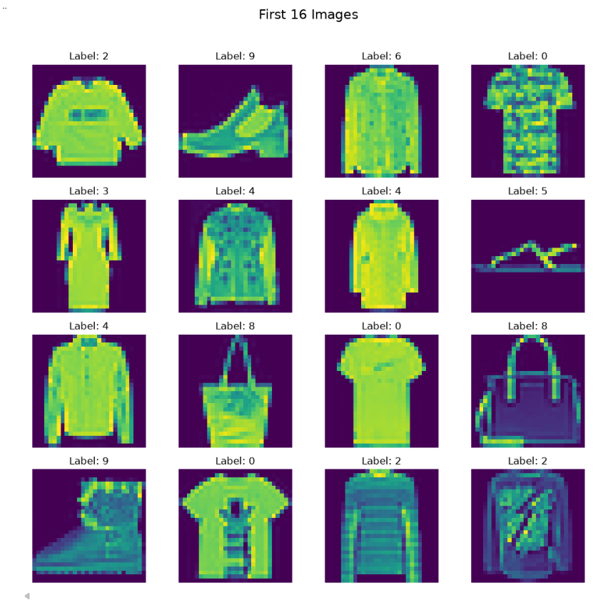
In Part 1 we built a network that recognises clothing. It worked — but it did something quietly insane, and I want to show you exactly what.

To feed a 28×28 image into that plain network, we flattened it: we took the grid of pixels and unrolled it into a single line of 784 numbers.

Stop and feel how strange that is. In the real image, a pixel knows its neighbours — a sleeve is a sleeve because of the pixels around it. The moment you flatten, that’s gone. Pixel #57 and pixel #58 were touching in the photo; in the flat line they’re just two entries with no memory that they were ever neighbours. We handed the network a jigsaw puzzle with all the pieces in a random pile and asked it to see the picture.

The astonishing part is that it still got decent accuracy. But we left a lot on the table. This post is about picking it back up.

The one idea to hold onto: a plain network throws away an image’s 2-D structure the instant it flattens it. A CNN keeps the structure — and that single change is usually the biggest accuracy jump you’ll ever get on images.

**▶️ Run the full CNN notebook →**

Quick bearings

If you’re arriving mid-series: every PyTorch project is the same 5 phases — Data → Model → Training → Tuning → Results — wrapped around one four-beat training loop (forward → measure → backward → update). That skeleton doesn’t change here. Almost everything in this post upgrades just one box: Phase 3, the model. (Plus one neat trick in Phase 2.) That’s the beauty of the mental model — you swap one part and the rest still fits.

What a convolution actually does

Instead of flattening, a CNN keeps the image as a 2-D grid and slides a tiny window — a filter (say 3×3) — across it, step by step. At each position the filter multiplies its little patch of pixels and produces one number: “how strongly does my pattern appear right here?”

That’s the whole trick. A filter is a small pattern-detector that sweeps the entire image. One filter might light up on vertical edges, another on curves, another on a patch of texture. And because the same filter is reused across every position, the network learns “an edge is an edge wherever it appears” — instead of relearning it separately for every location like the flat network had to.

Stack these layers and something beautiful emerges — a hierarchy:

• Early layers detect edges.
• The next combine edges into textures and shapes.
• Deeper ones assemble those into parts (a collar, a heel).
• The final ones recognise whole objects (shirt, sneaker).

In PyTorch that sliding filter is nn.Conv2d. You mostly give it how many filters to learn and their size, and it handles the sweeping.

Pooling: shrink, but keep what matters

After a convolution we usually pool. MaxPool2d(2, 2) looks at each 2×2 block and keeps only the strongest value, halving the width and height.

Why deliberately throw away three-quarters of the numbers? Two reasons: it keeps the salient signal while dropping noise, and it makes the network a little tolerant to small shifts — a sneaker nudged two pixels left is still a sneaker. Pooling is how a CNN says “I care that the edge is here, not the exact pixel.”

The anatomy: two stages

Zoom out and every CNN is just two stages bolted together:

1. Feature extraction — a stack of Conv → ReLU → BatchNorm → Pool blocks that distil the raw image into a small pile of rich feature maps.
2. Classification — flatten those feature maps and feed them into the same ordinary Linear layers from Part 1 to make the final 10-class decision.

So the CNN doesn’t replace what you learned — it bolts a smart image-reading front end onto the classifier you already understand.

🧠 Keep this sentence: convolutions find the features; the linear layers make the decision.

The one bit of arithmetic worth doing by hand

There’s a spot that trips up everyone: when you flatten the feature maps to hand them to the first Linear layer, what size are they? Get it wrong and you get a shape-mismatch error. It's worth tracing once, by hand, so it never mystifies you again:

Input:                 (1, 28, 28)    ← 1 grayscale channel
After Conv1 (32 filters, padding):  (32, 28, 28)   ← padding keeps size
After Pool1 (halves):               (32, 14, 14)
After Conv2 (64 filters, padding):  (64, 14, 14)
After Pool2 (halves):               (64,  7,  7)
Flattened:              64 × 7 × 7 = 3136 numbers → into the first Linear layer

Notice the pattern: convolutions (with padding) keep the size; only pooling shrinks it. Two poolings take 28 → 14 → 7. Trace it once and you’ll never fear that number again.

[IMAGE: the shape-tracing diagram (the notebook’s own cnn-shape-diagram.png works perfectly here)]

A free accuracy lever hiding in Phase 2: data augmentation

Here’s a technique that costs almost nothing and punches well above its weight. Before each training image reaches the model, we randomly perturb it — rotate it a few degrees, shift it slightly, occasionally mirror it:

train_transform = transforms.Compose([
    transforms.RandomRotation(10),                    # rotate up to ±10°
    transforms.RandomAffine(0, translate=(0.1, 0.1)), # shift up to 10%
    transforms.RandomHorizontalFlip(p=0.5),           # mirror sometimes
    transforms.ToTensor(),
])

Every epoch the model sees a slightly different version of each image, so it can never just memorise exact pixels — it’s forced to learn the general shape. It’s like turning one photo of a shirt into thousands of slightly-different shirts, for free.

Two honest caveats, because they’re the kind of thing tutorials skip:

• Augment the training set only. The test set stays pristine — it’s the exam, and you don’t rehearse on the exam.
• **RandomHorizontalFlip is questionable here.** A mirrored bag is still a bag, but mirroring can confuse asymmetric items. Sometimes removing it helps — augmentation is a knob, not a magic word.

Let the machine design the machine

We also carry over the Phase 3–4 defences from Part 1 — BatchNorm (now BatchNorm2d, the image-feature-map version), Dropout, and weight decay — and then do something a little wild.

Instead of hand-picking the architecture, we write the CNN with its depth and width as arguments (num_conv_layers, num_filters, fc_layer_size…) and hand the whole thing to Optuna. Across 50 trials it searches not just the learning rate but the shape of the network itself — how many conv layers, how many filters, how wide the classifier — hunting for the combination that scores best.

You stop guessing the architecture and let evidence pick it.

⚠️ Same honest caveat as Part 1: this notebook tunes on the test set, which mildly inflates the score. For real work, split off a validation set and keep the test set for one final, honest measurement. (The notebook’s closing section walks through this fix and nine others.)

What we actually changed

We didn’t learn a new framework or a new training loop. We swapped one box — the model — from “flatten and hope” to “keep the picture and slide filters across it,” added near-free augmentation in the data phase, and let Optuna design the rest. That’s the payoff of the 5-phase mental model: real upgrades are usually local.

Next time you see Conv2d, MaxPool2d, and a 64 * 7 * 7 in someone's code, you'll read it fluently: feature extractor, shrink step, flattened size going into the classifier.

▶️ Every layer, every shape, every Optuna trial — running:

👉 The full annotated CNN notebook →

📚 The whole series & code on GitHub →

📬 The Mental Model of PyTorch — a 5-part series

1. The Mental Model of PyTorch — Build a Neural Network in 5 Phases
2. Why Flattening an Image Throws Away the Picture — CNNs ← you are here
3. Don’t Train From Scratch: Standing on ImageNet’s Shoulders — transfer learning
4. Giving a Network Memory — RNNs and a Q&A bot
5. How Your Phone Keyboard Works — LSTMs, language modeling, and the door to Transformers

Next up → Part 3: why training from scratch is often the wrong move — and how to borrow a network that already learned to see.

Which idea clicked — the sliding filter, the shape-tracing, or the augmentation trick? Tell me below, and I’ll go deeper on it in a future post.