Finding Images by Color?

Have you ever scrolled through thousands of photos looking for that one sunset picture you took last summer? Or needed to find all the images with a specific color theme for a design project? Traditional search methods rely on manual tagging (metadata), but what if we could search based on the actual content of the images?

In this tutorial, I’ll show you how to build a simple but powerful image search system using color histograms. It’s one of the most intuitive approaches to content-based image retrieval (CBIR), and you’ll be amazed at how effective it can be with just a few lines of code!

What Are Color Histograms?

Think of color histograms as a fingerprint of an image based on its color distribution. Imagine taking all the pixels in an image, sorting them into color buckets, and counting how many fall into each bucket. This gives us a statistical representation of the image’s color profile that we can use to compare with other images.

For example, a beach scene would have lots of blue (sky/water) and yellow/tan (sand), while a forest scene would be dominated by greens and browns. By comparing these distributions, we can find visually similar images.

Let’s Build It!

We’ll implement our color histogram-based image search in Python using OpenCV. The code is provided in the accompanying notebook, but let’s walk through the key steps:

1. Loading and Processing Images

First, we’ll load some sample images. I’m using a dataset from HuggingFace, but you could use any collection of images:

from datasets import load_dataset
from base64 import b64decode
import cv2
import numpy as np

data = load_dataset('pinecone/image-set', split='train')
def process_image(sample):
    image_bytes = b64decode(sample['image_bytes'])
    image = cv2.imdecode(np.frombuffer(image_bytes, np.uint8), cv2.IMREAD_COLOR)
    return image
images = [process_image(sample) for sample in data]

# Since matplotlib reads it the other way
rgb_images = [np.flip(image, axis=2) for image in images]

2. Creating Color Histograms

Every pixel in each image has three BGR color values like this that range on a scale of 0 (no color) to 255 (max color). Using this, we can manually create RGB arrays to display colors with Matplotlib like so:

blue = [0, 0, 255]
green = [0, 255, 0]
red = [255, 0, 0]
violet = [255, 0, 255]
orange = [255, 165, 0]
yellow = [255, 255, 0]
cyan = [0, 255, 255]

colors = np.asarray([[blue, green, red, violet, orange, yellow, cyan]])

plt.imshow(colors)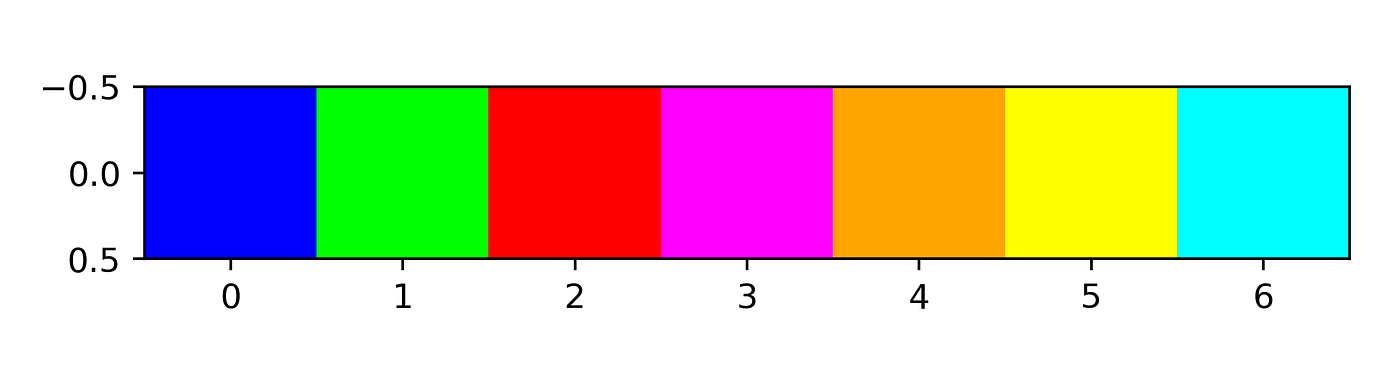

Here’s where the magic happens. We’ll extract a color histogram from each image:

def get_vector(image, bins=32):
    """Convert an image to a color histogram vector"""
    # Calculate histograms for each color channel
    blue_hist = cv2.calcHist([image], [0], None, [bins], [0, 256])
    green_hist = cv2.calcHist([image], [1], None, [bins], [0, 256])
    red_hist = cv2.calcHist([image], [2], None, [bins], [0, 256])

    # Concatenate all histograms ipnto a single vector
    vector = np.concatenate([red_hist, green_hist, blue_hist], axis=0)
    vector = vector.flatten()
    return vector

# Gotta astore the vector rep for all the images
image_vectors = []
for image in images:
    image_vectors.append(get_vector(image))

# If you want to view one of em! (But you gotta catch em all! ;)
image_vectors[0], len(image_vectors[0])

The bins parameter controls how fine-grained our color analysis is. With 32 bins per color channel, we end up with a 96-dimensional vector (32 bins × 3 channels) representing each image. This vector will have 96 dimensions, where values [0, … 32] are red, [32, … 64] are green, and [64, … 96] are blue.

3. Comparing Images

Now that we have our vectors, we need a way to compare them. Cosine similarity is a great choice for this:

Once we have these vectors we can compare them using typical similarity/distance metrics such as Euclidean distance and cosine similarity. In our case, we will be using cosine similarity.

def cosine_similarity(a, b):
    """Calculate cosine similarity between vectors a and b"""
    return np.dot(a, b) / (np.linalg.norm(a) * np.linalg.norm(b))

def euclidean(a,b):
  return np.linalg.norm(a-b)

4. Searching for Similar Images

Using our cosine function we can calculate the similarity which varies from 0 (highly dissimilar) to 1 (identical). We can apply this alongside everything else we have done so far to create another search function that will return the top_k most similar images to a particular query image specified by its index idx in images.

With our similarity metric in hand, we can now search for images that match a query:

def search(query_idx, top_k=5):
    """Find the top_k most similar images to the query image"""
    query_vector = image_vectors[query_idx]
    similarities = []
    for i, vector in enumerate(image_vectors):
        if i == query_idx:  # Skip the query image itself
            continue
        sim = cosine_similarity(query_vector, vector)
        similarities.append((i, sim))
    # Sort by similarity (highest first)
    similarities.sort(key=lambda x: x[1], reverse=True)
    # Return top k indices
    return [idx for idx, _ in similarities[:top_k]]

The Results: Seeing Is Believing!

Let’s see our search in action! I ran the search on a couple of query images and was impressed by the results:

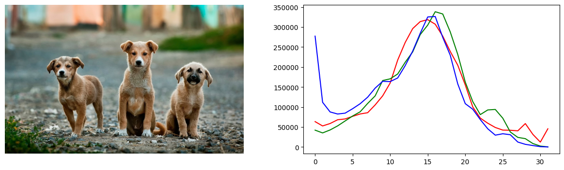
Fig. The image we want to query against our dataset and its color histogram

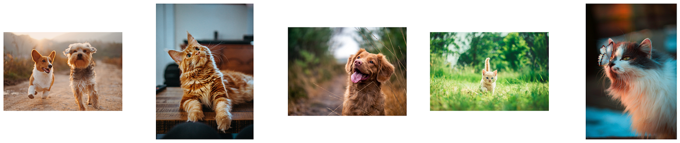
Fig. The top_k (5) most closely related images to the query image

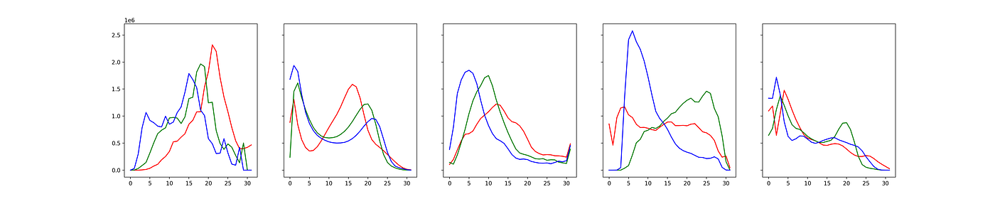
Fig. The color histograms of the top_k (5) most closely related images to our query image

1. When searching with an image of puppies, the system found other dog images with similar color profiles (as shown above).
2. With a city skyline at dusk, it returned other urban scenes with similar lighting.
3. Most interestingly, when I used an image with a vibrant yellow background, it found other images dominated by that same yellow tone!

What’s fascinating is that even though we’re only looking at colors (not shapes or objects), the results are often semantically meaningful. Images with similar color distributions frequently contain similar subjects or were taken in similar settings.

When to Use Color Histograms (and When Not To)

Color histograms shine in situations where color is a distinctive feature:

• Finding images with specific color schemes for design projects
• Organizing vacation photos by scenery type (beach vs. mountain vs. forest)
• Searching for visually similar product images

However, they do have limitations:

• They ignore spatial information (where colors appear in the image)
• They can’t distinguish between different objects with similar colors
• They’re less effective for B&W or low-contrast images

For more advanced image retrieval needs, deep learning-based approaches that understand semantic content would be more appropriate. But don’t underestimate the power of color histograms — they’re computationally efficient and surprisingly effective for many practical applications!

Bonus: Application to Medical Imaging

While our examples focused on everyday photos, similar histogram-based approaches have been used in medical imaging:

In medical scans, intensity distributions can indicate different tissue types or pathologies. For example, CT scans of healthy lungs have a different intensity histogram than those with pneumonia or nodules. By applying histogram analysis techniques, medical professionals or researchers enhance or normalize values depending on the equipement used, the reconstruction methods, organ, and so on.

Unlike regular photos, medical images often use grayscale intensities rather than color, but the principle remains the same — creating a statistical fingerprint of the image’s pixel values.

Here is a Python notebook to help you dive deeper into its medical imaging applications:

[embed]Medical-Image-Analysis/MedicalImg_Histogram_Analyses.ipynb at main ·… Jupyter Notebooks to help you understand medical imaging analysis with Python. …github.com

Final Thoughts

What amazes me about color histograms is how such a straightforward technique can yield such useful results. While modern deep learning approaches to image retrieval are incredibly powerful, they’re also complex and resource-intensive. Sometimes, elegant simplicity wins the day!

I encourage you to try this approach on your own image collection. Experiment with different numbers of bins and similarity metrics. You might be surprised at what you discover hiding in your photo library!

References

[embed]Color Histograms in Image Retrieval | Pinecone A look at one of the earliest content-based embedding methods.www.pinecone.io

[embed]examples/learn/search/image/image-retrieval-ebook/color-histograms/01-search-histogram.ipynb at… Jupyter Notebooks to help you get hands-on with Pinecone vector databases …github.com