How AI Learned to Render Photorealistic Worlds in Real-Time And What That Means for the…
NeRF is not a rendering technique. It’s a coordinate network trained on a differentiable image formation model. 3D Gaussian…
How AI Learned to Render Photorealistic Worlds in Real-Time And What That Means for the Rest of the Field
NeRF is not a rendering technique. It’s a coordinate network trained on a differentiable image formation model. 3D Gaussian Splatting is not a geometry method. It’s a set of explicit primitives optimized by a differentiable rasterizer using Adam. DLSS is not upscaling software. It’s a temporally-conditioned convolutional super-resolution model. The reason computer graphics suddenly started producing photorealistic images in real-time is that the entire field switched from hand-coded physics simulation to learned models and AI researchers have deep intuitions about exactly what changed and why.

A physically based path-traced render (Blender 3.0 Cycles). This image is best understood as a training target: a reference that physically correct light transport produces, and that neural rendering methods learn to approximate using gradient descent on differentiable image formation models. The question neural rendering answers is not “how do we compute this faster?” but “what function can a neural network learn such that its outputs are indistinguishable from this?” Image Credit: https://www.foxrenderfarm.com/share/what-is-path-tracing/
The Coordinate Network Nobody Called a Coordinate Network
In March 2020, Ben Mildenhall, Pratul Srinivasan, Matthew Tancik, Jon Barron, Ravi Ramamoorthi, and Ren Ng at UC Berkeley published a paper that the computer graphics community treated as a computer vision paper, the computer vision community treated as a graphics paper, and the machine learning community mostly ignored until a few months later, when someone noticed: this is just a coordinate network trained with a differentiable renderer.
The NeRF model (Neural Radiance Field) is an MLP that maps a 5-dimensional input to a 4-dimensional output:
F_θ(x, y, z, θ, φ) → (R, G, B, σ)That’s a position in 3D space, a viewing direction (azimuth and elevation), and the outputs are radiance (RGB color) and volume density σ. The scene its geometry, materials, and lighting is encoded entirely in the parameters θ of a 256-unit, 8-layer fully connected network. The training signal is photometric reconstruction loss between the network’s rendered output and real photographs of the scene.
This is structurally identical to a SIREN (Sitzmann et al., 2020), an occupancy network (Mescheder et al., 2019), or a coordinate MLP in any other neural implicit representation. The novelty was the differentiable image formation model volume rendering that allowed gradient descent to optimize θ from 2D image supervision alone, without 3D ground truth. The result was photorealistic novel view synthesis from ~100 photographs that generalized to camera positions no image had ever captured.
This is the paper that merged AI with photorealism. Every technique described in this article is either a derivative, an acceleration, or an extension of the core insight: 3D scene structure can be implicitly encoded in a neural function that is supervised differentiably through a rendering process.
Why MLPs Can’t Represent Scenes Without Fourier Features
The original NeRF paper’s most important architectural decision is easy to overlook in the excitement about novel view synthesis: positional encoding. The paper reports that removing it devastates reconstruction quality. Understanding why reveals something fundamental about using MLPs for continuous signal representation.
The problem is the spectral bias of neural networks (Rahaman et al., 2019; Tancik et al., 2020). MLPs trained with standard gradient descent preferentially learn low-frequency functions first and for natural scenes, the interesting detail (sharp edges, fine textures, specular highlights) lives in the high frequencies. A plain MLP given (x, y, z) coordinates learns a blurry, oversmoothed approximation of the scene.
The fix is random Fourier feature mapping (Tancik et al., NeurIPS 2020): embed the input coordinates into a higher-dimensional space using sinusoidal functions before passing them to the MLP.
# NeRF positional encoding
def positional_encoding(x, L=10):
    freqs = 2.0 ** torch.linspace(0, L-1, L)  # [L]
    x_enc = [x]
    for freq in freqs:
        x_enc.append(torch.sin(freq * torch.pi * x))
        x_enc.append(torch.cos(freq * torch.pi * x))
return torch.cat(x_enc, dim=-1) # input dim → 1 + 2L dimsWith L=10 frequency bands, a 3D coordinate (x,y,z) maps to a 63-dimensional vector. This gives the MLP access to a wide range of frequencies from the start the spectral bias no longer prevents learning fine-grained spatial detail because the high-frequency components are already present in the input representation.
The theoretical justification comes from the Neural Tangent Kernel perspective (Jacot et al., 2018): the effective kernel of an MLP maps to a stationary kernel over the input space, and the Fourier features shift the kernel’s spectrum to match the target signal’s frequency content. From an AI practitioner’s perspective: this is exactly the problem that also affects coordinate regression in other domains (neural audio synthesis, SDF-based geometry), and the Fourier embedding fix is broadly applicable.
NeRF’s positional encoding is the same random Fourier feature mapping used in approximate kernel methods for SVMs (Rahimi & Recht, 2007), repurposed as an input encoding for MLPs. The spectral bias of MLPs their tendency to prefer low-frequency functions appears in many neural representation problems and is generally addressed by the same class of input transformations.
Volume Rendering as a Differentiable Operation
The core of NeRF is not the MLP it’s the differentiable image formation model that allows backpropagation from pixel-space loss to MLP parameters. This is volume rendering, which computes the expected pixel color along a ray:
C(r) = ∫₀^∞ T(t) · σ(r(t)) · c(r(t), d) dt

where T(t) = exp(−∫₀ᵗ σ(r(s)) ds)
The accumulated transmittance T(t) captures how much light has passed through the scene from the camera to position t along the ray. σ is the volume density (how opaque the material is at each point). c is the view-dependent color (radiance) at each point given viewing direction d.
In practice, this continuous integral is approximated by stratified sampling: partition the ray into N intervals, sample one point per interval, and numerically integrate:
# Discrete volume rendering
def volume_render(colors, densities, deltas):
    # colors: [N, 3], densities: [N], deltas: [N] (interval widths)
    alphas = 1 - torch.exp(-densities * deltas)
    T = torch.cumprod(torch.cat([torch.ones(1), 1 - alphas[:-1]]), dim=0)
    weights = T * alphas  # [N] — contribution of each sample
    C = (weights.unsqueeze(-1) * colors).sum(dim=0)  # [3]
return CThis entire computation is differentiable with respect to colors and densities and colors and densities are outputs of the MLP so the entire chain from MLP parameters θ → ray samples → volume rendering → pixel color is differentiable. Standard MSE loss against training images provides gradients that flow all the way back to θ.
This is differentiable rendering: using a physically motivated but differentiable image formation model to supervise the neural representation from 2D image observations alone. No 3D supervision. No depth maps. No segmentation masks. Just posed RGB images and the differentiable renderer.
The loss is straightforward:
L = ||C_rendered - C_target||² + λ · L_regWhere L_reg can include sparsity on the volume density (to encourage a thin surface rather than cloudy volumes), distortion regularization (Mip-NeRF 360), or other geometric priors.
The training setup is remarkably similar to training an autoencoder: the “encoder” is the camera geometry (known from COLMAP structure-from-motion), the “latent” is the scene encoded in MLP weights θ, and the “decoder” is the differentiable renderer. Unlike an autoencoder, each scene requires a separate optimization there is no shared encoder across scenes in the original NeRF formulation.
Hash Encodings: Instant-NGP’s Architectural Insight
NeRF’s 100-hour training and 30-second per-frame rendering time are consequences of a specific architectural choice: encoding scene structure in MLP weights. Every time you query the scene at a new (x,y,z) position, you must run a forward pass through 8 fully-connected layers. For 192 samples per ray at 1080p resolution, that’s approximately 400 million MLP forward passes per frame.
Thomas Müller’s Instant Neural Graphics Primitives (NVIDIA, 2022) replace positional encoding with multiresolution hash encoding a learnable spatial feature store that the MLP decodes rather than encodes.
The hash table maintains F feature dimensions at T entries across L resolution levels, spanning minimum to maximum resolution:
# Simplified multiresolution hash encoding
class HashEncoder(nn.Module):
    def __init__(self, levels=16, features_per_level=2,
                 table_size=2**19, min_res=16, max_res=512):
        super().__init__()
        self.tables = nn.ParameterList([
            nn.Parameter(torch.randn(table_size, features_per_level) * 0.01)
            for _ in range(levels)
        ])

    def forward(self, x):  # x: [N, 3] in [0,1]
        features = []
        for level, table in enumerate(self.tables):
            resolution = self.resolution_at_level(level)
            # Hash the voxel corners at this resolution
            voxel = (x * resolution).long()
            idx = self.hash(voxel, len(table))
            # Trilinear interpolation of corner features
            feat = self.trilinear_interp(table[idx], x, resolution)
            features.append(feat)
        return torch.cat(features, dim=-1)  # [N, L*F]
The key properties:
(1). The hash tables are initialized randomly but optimized jointly with the MLP during training. The gradients from the scene’s photometric loss update the hash table entries, effectively teaching the spatial index to store useful features.
(2). Hash collisions different positions mapping to the same table entry are resolved in practice because the multi-resolution context disambiguates conflicting positions.
(3). The MLP receives rich spatial features from the hash encoder rather than raw coordinates, so it can be tiny (2–3 layers, 64 units) while still accurately decoding color and density.
The result: training time falls from 100 hours to 5 minutes on the same scenes, and rendering speed approaches real-time at reduced quality settings. The hash encoding trades compactness (original NeRF: ~5MB MLP) for speed (Instant-NGP: ~10–50MB hash tables + tiny MLP), a tradeoff that makes sense when render time is the bottleneck.
3D Gaussian Splatting: From Neural Fields to Differentiable Primitives
3D Gaussian Splatting: From Neural Fields to Differentiable Primitives 3D Gaussian Splatting (Kerbl et al., SIGGRAPH 2023) solves the NeRF inference bottleneck with a fundamentally different choice: replace the implicit neural field with explicit, differentiable 3D Gaussian primitives.
Each Gaussian primitive stores:
- μ ∈ ℝ³: 3D center position
- Σ ∈ ℝ^(3×3): 3D covariance matrix (encoding shape and orientation as an ellipsoid)
- α ∈ [0,1]: opacity
- c ∈ ℝ⁴⁵: spherical harmonic coefficients (15 per RGB channel, encoding view-dependent appearance)
The scene is represented as a cloud of N such primitives (N ≈ 1–6 million for typical scenes). To render, project all Gaussians to 2D, sort by depth, and alpha-composite. To train, backpropagate the photometric loss through the compositing operation.
The core mathematical operation projecting a 3D Gaussian to 2D: given 3D covariance Σ and camera Jacobian J (derived from the projection matrix), the 2D covariance is:
Σ_2D = J · W · Σ · W^T · J^Twhere W is the viewing transformation. This projection is analytic and differentiable.
The loss function is a combination of L1 and SSIM:
L_total = (1 - λ) * L1(render, target) + λ * (1 - SSIM(render, target))
# λ = 0.2 in the original paper
The SSIM term (Structural Similarity Index) penalizes structural differences in local patches more than L1 alone, which helps with recovering fine detail and sharp edges. This is the same loss combination used in many image reconstruction tasks it’s a standard choice for tasks where perceptual quality matters more than per-pixel accuracy.
Adaptive densification is the most algorithmically interesting component. During training, the optimizer monitors the gradient magnitude at each Gaussian’s position. Gaussians in regions with high reconstruction loss and high positional gradient get either split (Gaussian with large covariance split into two smaller ones) or cloned (duplicate placed nearby with smaller scale). Gaussians that become too transparent (opacity below threshold) are pruned. This adaptive mechanism is why 3DGS achieves such high quality without a fixed geometry representation the Gaussians organize themselves to match the scene’s structure.
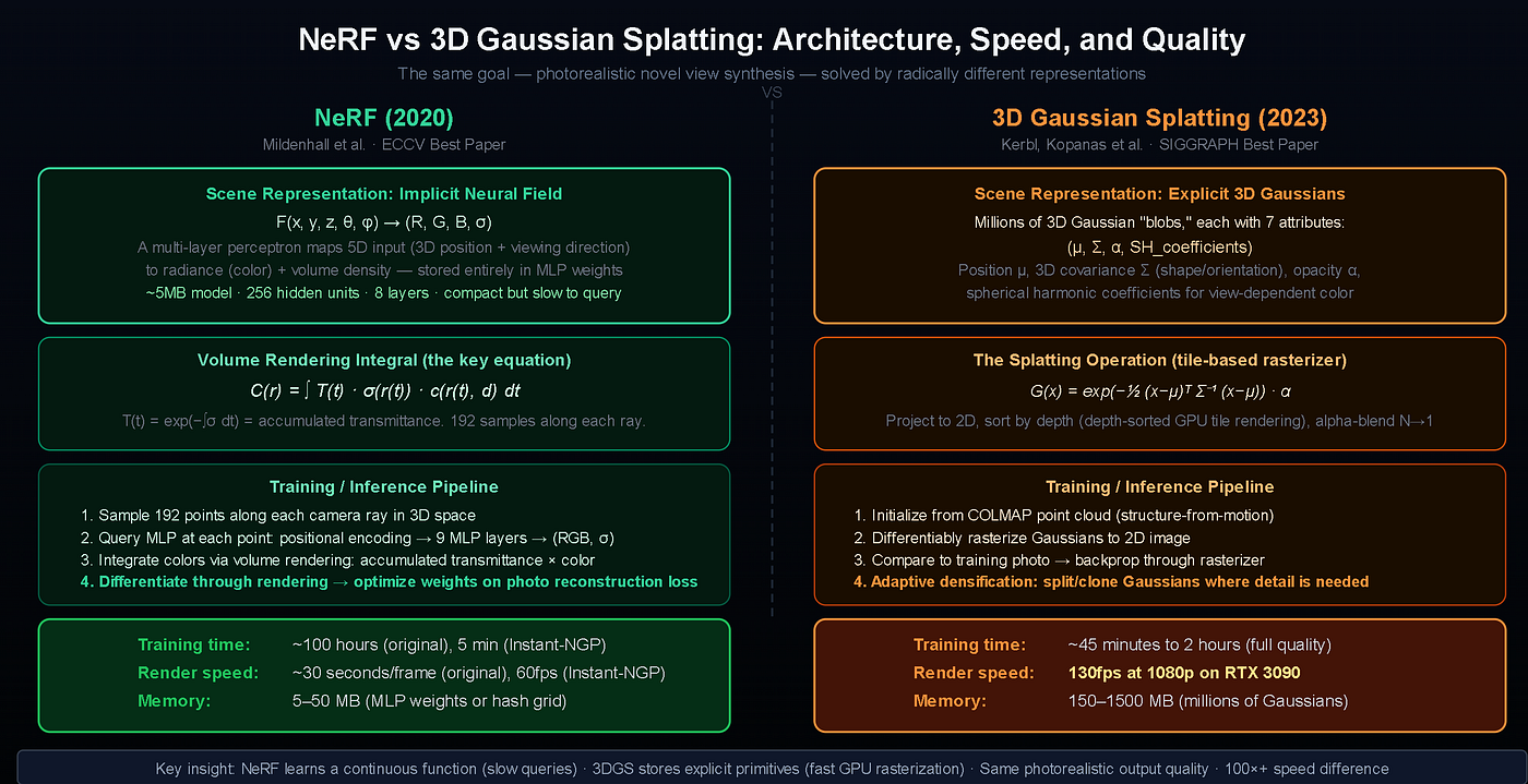
NeRF vs 3D Gaussian Splatting two different answers to the same question. NeRF encodes scenes in MLP weights and renders by numerically integrating along rays. 3DGS stores millions of explicit Gaussian blobs and renders by GPU-accelerated differentiable rasterization. Both are trained with gradient descent on photometric reconstruction loss. Speed difference: 30 seconds/frame (NeRF original) vs 130fps (3DGS, RTX 3090). Image Credit: Original diagram created for this article.
The inference speed advantage comes directly from the explicit representation: rendering 3DGS requires no neural network inference just GPU-accelerated Gaussian rasterization, which maps exactly to operations modern GPUs are optimized for. 130fps at 1080p on an RTX 3090 is the headline number from the original paper; subsequent work (RadSplat, 2024) has reached 900+ fps.
The Training Objectives: What These Models Actually Learn
The quality of neural rendering depends heavily on the training objective. Across NeRF, Instant-NGP, and 3DGS, the loss function choice has evolved to better capture perceptual image quality.
L2 (MSE) loss is the mathematically simplest choice: minimize mean squared error in pixel space. It’s tractable, has clean gradients, and is implicitly maximizing PSNR. The problem: L2 penalizes any deviation equally regardless of spatial structure, so it tends to produce blurry outputs when there is any ambiguity or noise in the training signal. High PSNR doesn’t always mean high perceived quality.
SSIM (Structural Similarity Index) captures local structural coherence. It computes similarity over local patches using luminance, contrast, and structural comparison. SSIM loss encourages the model to preserve local structure even when per-pixel values drift. Most 3DGS variants use L1 + SSIM.
LPIPS (Learned Perceptual Image Patch Similarity), Zhang et al. 2018, computes feature-space distance using a pretrained VGG or AlexNet. This directly optimizes for perceptual quality what humans can distinguish rather than per-pixel accuracy. LPIPS produces sharper, more realistic outputs than L2 at the cost of potential hallucination of plausible but incorrect detail. Widely used in generative modeling; less common in NeRF (because hallucination of detail that wasn’t in training images is undesirable for reconstruction).
Depth supervision from monocular depth estimation (DPT, ZoeDepth) adds geometric grounding when training images are sparse. The depth estimator provides a “soft prior” on scene geometry that helps disambiguate 3D structure from limited viewpoints connecting neural rendering to the broader monocular depth estimation literature.
Score Distillation Sampling: Diffusion Models as 3D Loss Functions
The most remarkable recent development in neural rendering from an AI architecture perspective is Score Distillation Sampling (SDS), which uses a pretrained text-to-image diffusion model as a loss function for optimizing a 3D neural representation.
DreamFusion (Poole, Jain, Barron, Mildenhall, ICLR 2023) posed the problem: given a text prompt, optimize a NeRF such that rendered views from any angle look like they were generated by a diffusion model conditioned on that text. The training signal comes entirely from the diffusion model no 3D dataset needed.
The SDS gradient with respect to NeRF parameters θ is:
∇_θ L_SDS = E_{t,ε} [w(t) · (ε_φ(z_t; y, t) - ε) · ∂x/∂θ]Where:
- z_t is a noisy latent (rendered image + noise at timestep t)
- ε_φ(z_t; y, t) is the diffusion model’s predicted noise given text condition y ε is the actual noise that was added
- w(t) is a weighting schedule
- ∂x/∂θ is the Jacobian of rendered pixels with respect to NeRF parameters
The gradient tells the NeRF: “change your parameters in the direction that makes this rendered view look less like a noisy version of text-conditioned images.” The diffusion model, trained on billions of text-image pairs, provides a prior that any view of a “red car” (or whatever the prompt specifies) should be consistent with its training distribution. Backpropagating this signal through the differentiable renderer optimizes the 3D structure to match that prior.
DreamGaussian (Tang et al., 2023) extends DreamFusion by replacing the NeRF with 3D Gaussian Splatting as the differentiable 3D representation, dramatically accelerating text-to-3D optimization from hours to minutes.

Magic3D (Lin et al., 2022) demonstrates text-to-3D via Score Distillation Sampling. The diffusion model acts as a “prior” over how text-described 3D objects should look from any viewpoint, providing gradient signal through differentiable rendering to optimize a neural 3D representation. This is structurally identical to any other form of distillation the diffusion model is the teacher, the 3D representation is the student but operates entirely in the rendering loop rather than in weight space. Image Credit: Lin et al., 2022 · via MarkTechPost · marktechpost.com
SDS has known failure modes that connect directly to the broader generative modeling literature. Mode collapse: the optimizer finds renders that maximally satisfy the diffusion prior but are geometrically inconsistent the “Janus problem” where a face appears on all sides of a head. Over-saturation: SDS tends to produce over-saturated, cartoonish outputs because it optimizes toward the mode of the diffusion distribution rather than sampling from it. Variational Score Distillation (VSD, Wang et al., 2023) addresses this by treating the 3D representation as a distribution and using a particle-based variational approach, connecting SDS to the score matching literature.
The Classical Pipeline Rasterization’s Limits Seen Through an AI Lens
To understand why neural methods were needed, consider what rasterization does from a function approximation perspective.
Rasterization computes, for each pixel, the color of the nearest surface visible from that pixel, using a hand-coded shading model (Phong, PBR) that takes surface normals, material parameters, and light positions as input. This is a closed-form approximation to the rendering equation that ignores all light paths that bounce between surfaces before reaching the eye.
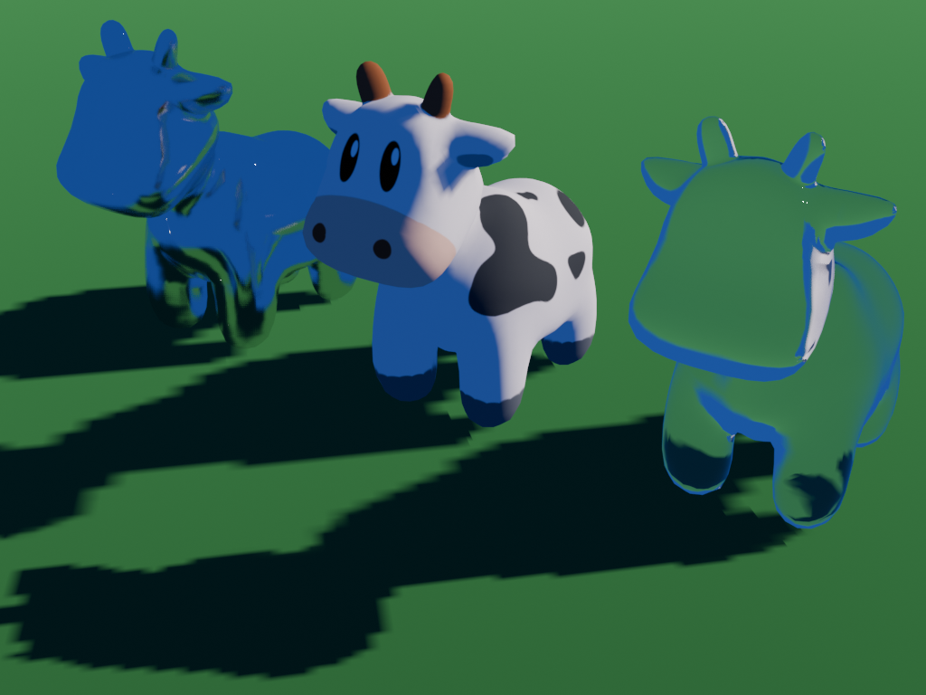
Rasterization (Blender EEVEE) a first-order approximation to light transport. Physically, the color at each pixel is an integral over all possible light paths connecting light sources to that pixel. Rasterization approximates this by considering only the direct path (one bounce). The visible consequences — flat lighting without color bleeding, hard shadow edges, no inter-reflections are systematic approximation errors, not implementation failures. Image Credit: Blender Foundation · Wikimedia Commons · commons.wikimedia.org · License: CC BY 4.0
Ray tracing computes more bounces of the light integral, it is a better approximation but still noisy at limited samples.

The Cornell box rendered by BMRT path tracer. The color bleeding on the ceiling from red and green walls is the visible signature of multi-bounce light transport exactly the signal that makes renders look photorealistic. This scene serves as ground truth; neural denoisers are trained on pairs of (1spp noisy, 4096spp clean) Cornell-box-style renders and must reconstruct the color bleeding from the noisy single-sample observations. Image Credit: Larry Gritz / BMRT · Wikimedia Commons · Public Domain
The neural rendering pipeline we now use is: rasterize primary visibility fast → ray trace 1 sample per pixel for global effects → neural denoise to simulate 64spp quality → neural upsample to 4K resolution. Each neural component learns to approximate the result of more expensive computation.

The complete real-time neural rendering pipeline. From an ML perspective: the denoiser is a U-Net trained on noisy→clean image pairs with auxiliary buffers (albedo, normals, depth) as conditioning inputs. The DLSS upsampler is a temporally-conditioned CNN trained to infer 4K resolution from 1080p input and prior frames. Both are inference-only during game rendering; training happens offline on NVIDIA’s supercomputing clusters. Image Credit: Original diagram created for this article.
Neural Denoising as a Supervised Regression Problem
Monte Carlo denoising is, from an ML perspective, a conditional image-to-image regression problem. The input is a noisy, 1-sample-per-pixel path-traced render with auxiliary G-buffers (albedo, normal, depth). The output is a denoised version that should match the result of running many more samples.
The training setup:
- Dataset: Pairs of (1spp render + G-buffers, reference 4096spp render) on diverse scenes
- Architecture: Primarily U-Net based (NVIDIA OptiX denoiser, OIDN) with skip connections between encoder and decoder. Recent versions add attention mechanisms
- Loss: L2 in HDR pixel space, sometimes with perceptual component Conditioning: G-buffers enter as additional channels alongside the noisy color input
The G-buffers are critical. The albedo buffer (surface color without lighting) tells the denoiser what color the surface should be, disambiguating noise from genuine surface color variation. The normal buffer tells it surface orientation, helping distinguish hard edges from noisy gradients. The depth buffer provides geometry context for determining what’s near vs far.
NVIDIA’s DLSS Ray Reconstruction (2023) extends this with temporal accumulation: the denoiser also receives the denoised previous frame (warped to the current viewpoint), allowing it to exploit temporal coherence. This is the same principle as recurrent denoising autoencoders in video (Chaitanya et al., SIGGRAPH 2017) adjacent frames in a video share most of their content and differ only in motion.

Path-traced glass caustics one of the hardest denoising targets. The caustic pattern (bright focused light on the floor) is created by rays that pass through the glass, refract, and focus. At 1spp, each pixel either catches a caustic ray (bright) or doesn’t (dark), creating an extremely noisy estimate of a sharp signal. Neural denoisers learn to recognize the statistical signature of these patterns and reconstruct their expected appearance. Image Credit: https://www.foxrenderfarm.com/share/what-is-caustic-in-optics/Resolution
DLSS (Deep Learning Super Sampling) is a specific application of neural image super-resolution with temporal information. The AI architecture perspective:
DLSS 1 (2018): a single-frame CNN upsampler trained on synthetic data, comparable to ESRGAN but with less temporal stability.
DLSS 2 (2020): reframed the problem as temporal super-resolution. Instead of upsampling a single frame, accumulate information across frames. The architecture accepts the current low-resolution frame + motion vectors (optical flow from the game engine) + the previous high-resolution frame (warped to current viewpoint). A transformer-based network reconstructs 4K resolution by combining current low-res information with temporally accumulated high-res detail.
DLSS 3 (2022): Frame Generation. Generate an entirely new frame between two rendered frames using optical flow interpolation + a trained refinement network. This doubles the effective framerate one rendered frame, one generated frame. The generated frames are not truly rendered: they interpolate between rendered states, so they can miss frame-accurate response to player input (hence the latency concern).
DLSS 4 (2025): Multi Frame Generation generate 3 frames for every 1 rendered, quadrupling effective framerate. The network learns an optical flow prediction + appearance refinement model trained on game-engine-rendered sequences, and generates photorealistic intermediate frames at inference time.
From a video generation perspective, DLSS 4’s Multi Frame Generation is structurally related to video interpolation models (FILM, RIFE, AMT) but trained on a more constrained domain (game renders with available depth and motion vectors as conditioning) and optimized aggressively for inference latency (<2ms on RTX 50-series hardware).
NeRF Beyond Novel View Synthesis: Scene Representations for AI
For AI researchers, the most significant consequence of the NeRF literature may not be photorealistic rendering at all, it’s the emergence of neural radiance fields as general-purpose scene representations for AI applications.
Feature Fields / Language-Embedded Radiance Fields (LERF): Kerr et al. (2023) embed CLIP feature vectors into a radiance field alongside RGB, creating a 3D representation where every point has both appearance (color/density) and semantic content (CLIP embedding). Given a text query (“the red cup”), you can localize objects in 3D space by finding the regions with highest CLIP-text similarity. This extends open-vocabulary understanding to 3D without explicit 3D segmentation.
Scene representations for robotics manipulation: Gaussian Splatting and NeRF provide dense, photorealistic scene models that robots can use for task planning, grasp point estimation, and trajectory optimization. Huang et al. (2023) show that a NeRF trained on a robot workspace can provide photorealistic simulation for evaluating grasping policies without physical trials using the differentiable renderer to optimize grasp poses that maximize visual consistency with success criteria.
World models for RL: A world model is a learned simulator: given a state and action, predict the next state. NeRF provides a photorealistic world model for visual observations a robot or autonomous agent can simulate “what would I see if I moved left” by querying the NeRF from the new viewpoint. This is directly compatible with Dreamer-style (Hafner et al.) model-based RL, where the agent imagines trajectories in the world model and learns policies from those imagined experiences.
Generalization to novel scenes: The single-scene NeRF limitation (train a new model from scratch for each scene) is addressed by generalizable NeRF models that condition on a few reference images. Large Reconstruction Model (LRM, Hong et al., 2023) uses a transformer encoder-decoder to produce a NeRF from a single image in ~5 seconds moving toward zero-shot 3D scene understanding without per-scene optimization.
The Open Research Problems (Through an AI Lens)
Dynamic scene reconstruction: NeRF and 3DGS represent static scenes. Dynamic scenes require either (a) time-conditioned representations (add t as an input coordinate), (b) deformation fields (learn a canonical scene + deformation network), or © 4D Gaussian Splatting (optimize time-varying Gaussian positions). None of these scale to arbitrary real-world dynamics at real-time quality. 4DGS (Wu et al., 2024) demonstrates the concept; production-quality real-time dynamic neural rendering remains open.
Single-image or sparse-view generalization: LRM-style feedforward 3D generation from 1–4 images is advancing rapidly (Zero123, Zero-1-to-3, InstantSplat) but still produces artifacts on complex scenes. The fundamental challenge is that 3D reconstruction from very few views is heavily under-constrained it requires strong learned 3D priors that current architectures only partly capture.
Unbounded outdoor scenes: Mip-NeRF 360 and 3DGS with floaters-pruning address bounded outdoor scenes, but city-scale reconstruction (hundreds of square kilometers from aerial imagery) requires hierarchical representations, streaming LOD (Octree-GS, HiGS), and distributed training that are all active research areas.
Composition and editability: After training, NeRF and 3DGS are difficult to edit (move an object, change a material, add a light source). Segmenting scenes into object-level representations and editing them in a principled way while maintaining photorealism is an open problem with connections to instance segmentation, compositional generative modeling, and inverse rendering.
Combining with diffusion for coherent generation: DreamFusion and friends produce 3D objects, but large-scale scene generation (a whole room from a text prompt, or a city from a satellite view) requires combining neural rendering with generative models at a scale that current compute budgets don’t support at interactive quality.
The Unified View: What This Means for AI
The neural rendering field has, in five years, replaced most of classical computer graphics’ core algorithms with learned models. The pattern is consistent: take a physically motivated but computationally expensive operation, replace it with a neural function trained on the expensive operation’s outputs, and recover most of the quality at a fraction of the cost.
This is exactly the “distillation from physics simulators” template that appears across AI. Molecular dynamics → learned force fields. Computational fluid dynamics → neural PDE solvers. Protein structure from first principles → AlphaFold. In each case, the neural model learns to reproduce a expensive physical computation at inference speed.
Neural rendering adds one additional ingredient: differentiable simulation. The rendering model is not just learned from expensive simulations, it is itself differentiable, which means it can be optimized end-to-end as part of larger systems. NeRF trained with SDS is a 3D representation optimized against a text-to-image model’s distribution. Gaussian Splatting trained in a robot workspace is a scene model optimized against manipulation success criteria. This is the direction the field is moving: neural rendering as a differentiable component in larger AI pipelines, not as a standalone rendering technology.
For AI practitioners, the practical takeaway is that 3D scene representation is no longer a problem that requires specialized graphics expertise to approach. The tools (NeRF implementations in PyTorch, gsplat, nerfstudio), the training pipelines, and the loss functions are all standard ML infrastructure. The research problems that remain dynamic scenes, generalization, scale, editability are ML research problems with graphics priors attached, not graphics problems with ML solutions bolted on.
Where to Go From Here
- NeRF: Representing Scenes as Neural Radiance Fields
- 3D Gaussian Splatting for Real-Time Radiance Field Rendering
- DreamFusion: Text-to-3D using 2D Diffusion (SDS paper)
- gsplat: Open-source Gaussian Splatting in PyTorch
- nerfstudio: Modular NeRF framework
- Instant-NGP (NVIDIA): Multiresolution Hash Encoding
- LERF: Language Embedded Radiance Fields
- Mip-NeRF 360: Unbounded Anti-Aliased Neural Radiance Fields
References
메타데이터
- post_id
- 41358a1f683a
- slug
- how-ai-learned-to-render-photorealistic-worlds-in-real-tim-e-and-what-th-at-means-for-the-41358a1f683a
- url
- https://ai.gopubby.com/how-ai-learned-to-render-photorealistic-worlds-in-real-tim-e-and-what-th-at-means-for-the-41358a1f683a
- canonical_url
- https://ai.gopubby.com/how-ai-learned-to-render-photorealistic-worlds-in-real-tim-e-and-what-th-at-means-for-the-41358a1f683a
- author_url
- https://medium.com/@hayanan
- status
- ok
- fetched_at
- 2026-07-09 03:40:04