How to Estimate resources for Training and Serving Large Language Models

Training or serving a large language model requires a large amount of compute, memory, and communication bandwidth. These requirements can look difficult to estimate at first because many details are involved: model architecture, number of parameters, sequence length, batch size, hardware, and numerical precision.

In this post, I will describe practical formulas for estimating the resources needed for both training and inference. The goal is not to produce a perfect simulator of every kernel and every hardware detail. The goal is to build a reliable first-order estimate. This estimate is useful when choosing a model size, planning a training run, or understanding how many requests an inference server can handle.

Training

Training cost can be estimated step by step: first we choose the model size and the number of training tokens, then we use these values to estimate total FLOPs, then we calculate memory for weights, gradients, optimizer states, and activations, and finally we estimate training time.

Compute-optimal Chinchilla rule

Scaling laws presented in the *Chinchilla *paper from DeepMind describe how model quality changes when we increase training compute, model size, and dataset size.

A common takeaway is that for a standard transformer, optimal performance is achieved by training on roughly 20 tokens per parameter.

Compute FLOPs

The classic training compute approximation is:

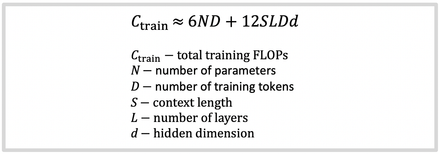
Why 6ND?

Forward

A single linear layer can be written as:

For each token, the forward pass costs roughly 2N. Because this matrix multiplication has N multiplications and approximately N additions.

A transformer is a stack of many such linear layers (attention, output, and feed-forward projections). If we sum over all linear layers, the forward pass costs roughly 2N FLOPs per token.

Backward

Backward training costs about twice the forward pass: gradient with respect to W and gradient with respect to X. It costs 4N per token. So the forward-plus-backward costs 6N per token.

Why 12SDLd?

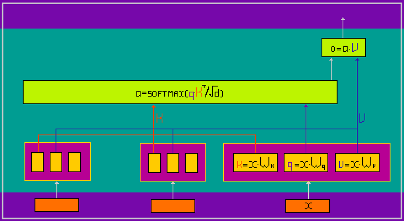
Attention with respect to a single token

The term 12SDLd is the sequence-length-dependent training cost of self-attention per token, 4SDLd comes from the forward attention matmuls:

And the factor 3 converts forward cost into forward-plus-backward training cost. This part of the formula becomes important when the context size is large.

The whole formula counts the dominant forward-and-backward model matmuls. It is a first-order estimate and usually excludes optimizer update FLOPs and parameter-update overhead; this omission is usually acceptable for large-batch training, because the optimizer cost is paid once per step, while the forward and backward cost scales with all tokens in the batch, so the optimizer contribution per token becomes relatively small.

Training memory

Training memory is usually the hard limit. Total training memory is roughly:

Memory for states

The common formulas are:

For mixed-precision Adam, a common estimate is:

bf16/fp16 weight = 2 bytes
bf16/fp16 gradient = 2 bytes
fp32 master weight = 4 bytes
fp32 Adam momentum m = 4 bytes
fp32 Adam variance v = 4 bytes
---------------------------------
Bytes per parameter = 16 bytes
Total = 16N

So a 7B model needs roughly 16 × 7e9 = 112 GB.

Memory for activations

During training, the model must store intermediate values from the forward pass because they are needed later during the backward pass. These intermediate values are called activations.

For example, activations are needed for weight gradient computation in linear layers.

Activation memory is different from weight memory. Weight memory depends mainly on the number of model parameters. Activation memory depends mainly on the batch size, sequence length, hidden size, number of layers, and implementation details.

A useful high-level estimate is:

In *Reducing Activation Recomputation in Large Transformer Models* paper the authors arrived at the following approximate formula for transformer architecture:

For a 7B model, distribution of memory components could look like this at training time:

N = 7e9, L = 32, d = 4096, H = 32, B = 4

There is a **FlashAttention algorithm, which reduces the activation memory**, especially at long sequence length, because the attention quadratic tensors no longer need to be kept in GPU memory across the forward-to-backward boundary:

The tradeoff is extra recomputation in backward.

N = 7e9, L = 32, d = 4096, H = 32, B = 4, FlashAttention

With activation checkpointing, you can store fewer activations and recompute them during backward pass. This technique reduces training memory by not storing all forward activations until the backward pass. Instead, the training system saves only a selected subset of tensors, called checkpoints, and recomputes the missing intermediate activations when they are needed during backpropagation. This changes the memory estimate because the activation term becomes smaller, while the total training compute and step time increase due to the extra recomputation. In other words, gradient checkpointing trades memory for compute.

Inference

Inference has a different cost structure. During inference, we do not store gradients or optimizer states, and the model does not need to keep large activation tensors for backpropagation, so activation memory is much smaller than during training. But inference has its own bottlenecks. The KV-cache can become very large when many users are served at the same time or when the context length is long. The decode stage is often limited by memory bandwidth rather than raw FLOPs.

Inference has two phases:

1. Prefill: process the prompt.
2. Decode: generate new tokens one at a time

Compute FLOPs

Prefill FLOPs can be estimated similarly to a training step forward pass:

For generating one new token for sequences in a batch of size B at current context length S:

Inference memory

Total serving memory is roughly:

Memory for weights

A 7B model in bf16 needs 7e9 × 2 = 14 GB.

Memory for KV-cache

During autoregressive inference, the model generates one new token at a time. At each layer, self-attention needs the keys and values of all previous tokens in the current context. Recomputing these tensors from scratch at every decoding step would be very expensive, so inference systems store them in memory after they are produced. This stored memory is called the KV-cache.

For each new token, the model computes its new key and value vectors, appends them to the cache, and then attends over the full set of cached keys and values. This makes decoding much faster because previous tokens do not need to pass again through the key and value projections. However, the KV-cache can become one of the largest memory costs during serving, especially for long contexts or large batches. Its size grows linearly with the number of layers, the hidden size of the key and value projections, and the total number of cached tokens.

Several techniques can reduce the KV-cache cost. The most direct architectural change is to reduce the number of KV heads: multi-query attention (MQA) shares one key-value head across all query heads, and grouped-query attention (GQA) shares one KV head across a group of query heads. A second method is to limit how much past context must remain in the cache: sliding-window attention keeps only a local window of previous tokens instead of attending to the full history, which changes the effective cache growth from full-context storage to window-limited storage. A third method is KV-cache quantization, which stores keys and values in fewer bits and can substantially reduce memory footprint, although aggressive quantization may hurt quality if it is not done carefully. Finally, systems such as PagedAttention do not reduce the theoretical KV-cache size in the formula itself, but they reduce fragmentation and wasted allocation, which lowers the practical memory overhead of serving.

Memory for activations

*Mtmp_act represents temporary forward-pass memory. It includes hidden states, attention intermediates, and kernel-local workspaces. Unlike model weights, it is not fixed. Unlike the KV-cache, it does not remain after the current forward pass finishes. It is usually much smaller than Mweights for large models and smaller than Mkv* at long context lengths.

A practical estimate is the maximum live activation size inside one layer during prefill stage (with FlashAttention):

For a 7B model, the distribution of memory components could look like this at inference decoding time:

N = 7e9, L = 32, H = 32, dhead=128, B = 4, bkv=2, FlashAttention

MoE corrections to the estimates

For a mixture-of-experts model, the dense formulas should be corrected by separating total parameters from active parameters: in standard LLM-style MoE models, the attention layers remain dense while the FFN layers are replaced by experts, and only a small number of experts are selected for each token.

• Compute FLOPs should be estimated from the active parameters, not from the full parameter count, because only the routed experts are executed for each token.
• Weight memory scales with the total stored parameters, because all experts must exist in memory even if they are not used by the current token. Optimizer-state memory and checkpoint size follow the same rule during training.
• Activation memory scales with the active experts plus router and dispatch buffers, not with all experts at once.
• KV-cache memory is unchanged compared with a dense model

Conclusion

Estimating the cost of an LLM becomes much easier once we separate the problem into a few basic components. For training, the main questions are how many parameters to use, how many tokens to train on, how much memory is needed for weights, gradients, optimizer states, and activations, and whether the total step time is limited by computation or communication. For inference, the structure changes: weights become a fixed memory cost, the KV-cache grows with context length, and decoding is often limited by memory bandwidth rather than pure FLOPs. You can find more information about identifying bottlenecks in computing, data handling, and data transfer during different parallelization schemes in the guides *“How to Scale Your Model” and “The Ultra-Scale Playbook”. You can also read my post “Visualization of Data Parallelism for LLM Training: From Naive Data Parallelism to ZeRO-3”* where I tried to explain algorithms with detailed pictures.

The formulas in this post give a practical way to reason about these costs before running expensive experiments. Of course, real systems add extra details such as kernel efficiency, communication overhead, quantization, and parallelism strategy. But the first-order estimates are still useful.

Links

• Chinchilla paper from DeepMind
• Reducing Activation Recomputation in Large Transformer Models paper
• Flash Attention paper
• “How to Scale Your Model” guide with JAX code examples
• The Ultra-Scale Playbook with an introduction in different types of parallelization.
• Visualization of Data Parallelism for LLM Training: From Naive Data Parallelism to ZeRO-3